Statistical Analysis: Modelling the Effect of Communicative Attempt (H1) and Answer Similarity (H2) on Effort
Overview
In this script, we will be modelling the causal relation between effort and correction to confirm/reject our hypothesis.
These are:
H1: In corrections, people enhance some effort-related kinematic and/or acoustic features of their behaviour relative to the baseline.
H2: The enhancement depends on similarity of the guesser’s answer and the original meaning. More similar answer will require/result in smaller enhancement (but still enhancement) than less similar answer.
To assess the design and performance of the model, we will use synthetic data that we create to have certain interdependencies and where the effects have pre-defined values. We use this approach instead of using our dyad 0 data, because the pilot data do not include enough data to have a sensible testing sample.
The confirmatory analysis concerns six outcome variables, namely integral of torque change, integral of amplitude envelope, integral of change in center of pressure, and mean peak value of torque change, mean peak value of amplitude envelope, and mean peak value of change in center of pressure.
For our exploratory analysis, we will model variables that will result as most predictive in relation to communicative attempt, assessed by XGBoost modelling. This is why in our synthetic data, we create a variable Effort that is continuous, but oterwise free of any other assumptions.
Code to prepare the environment
library(here)library(dplyr) # for data-wranglinglibrary(tidyr) # for reshaping data (if needed)library(ggplot2)library(tibble)library(rcartocolor)library(patchwork)library(ggdag) # for daglibrary(dagitty)library(bayesplot) # bayesian stufflibrary(brms)library(beepr)library(bayestestR)library(tidyverse)library(splines) # for bsplineslibrary(emmeans) # for lognormal transformations# current folder (first go to session -> set working directory -> to source file location)curfolder <-getwd()parentfolder <-dirname(curfolder)featurefolder <-paste0(parentfolder, '/07_TS_featureExtraction/Datasets/')demofolder <-paste0(parentfolder, '/00_RAWDATA/Demographics_all/')datasets <-paste0(curfolder, '/datasets/')models <-paste0(curfolder, '/models/')plots <-paste0(curfolder, '/plots/')
Loading in our data
This is the feature dataframe we will be using when having access to full data. Additionally, we will merge the feature dataframe with demographic data collected via Qualtrics.
For confirmatory analysis, we will need only 6 features - arm torque integral, arm torque peak mean, COPc integral, COPc peak mean, envelope integral and envelope peak mean from the data_feat. From data_demo, we will need only BFI and Familiarity
To merge them, we will need to have column pcn_ID in data_feat too.
# Extract participant part from TrialIDdata_feat <- data_feat %>%mutate(pcn_ID =str_extract(TrialID, "^[0-9]+") %>%# Extract first number (before first underscore)paste0("_", str_extract(TrialID, "p[0-9]+") %>%str_remove("p")) # Extract last part and format as pcn_ID )final_data <-left_join(data_feat, data_demo, by ="pcn_ID")head(final_data, n=15)
Because current pilot data are quite likely unsufficient in terms of power (65 observations), and would hinder testing the design of the statistical models, we will create synthetic data with assumed coefficients for all predictors we plan to add to the model.
H1: Stating causal model
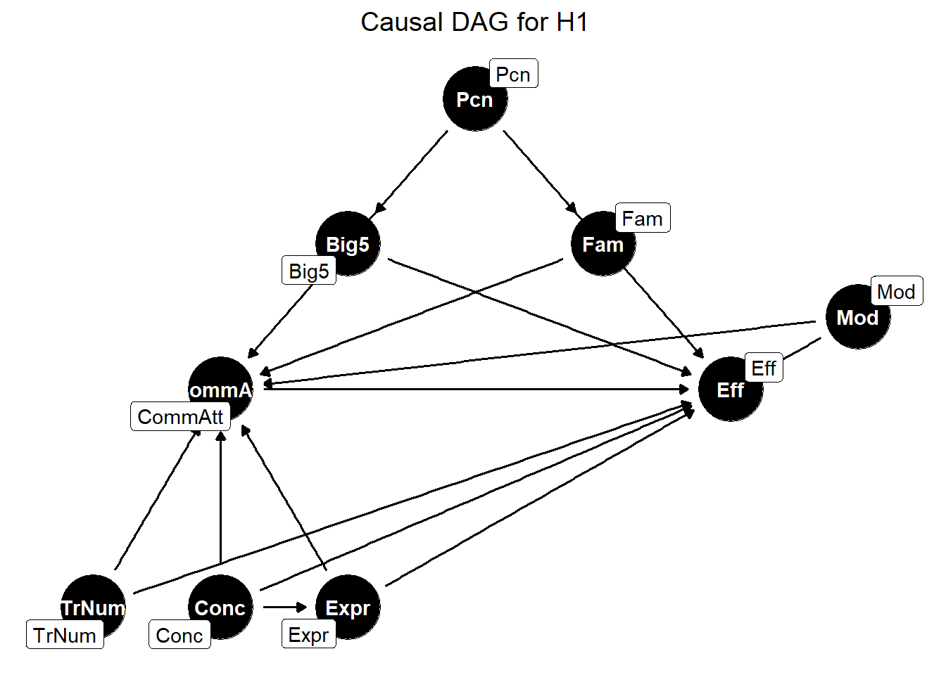
Before simulating synthetic data, we will first formulate our causal model to explicitly identify common causes, and hence prevent (or rather minimize) confounding in our statistical model. Note that while we are interested in causal relationship between effort (outcome) and communicative attempt (predictor for H1) and answer similarity (predictor for H2), we need to acknowledge that there are other factors possibly contributing to the outcome variable, despite the experiment beling relatively controlled. These relate, for instance, to the participants (e.g., personality traits) or stimuli (i.e., concepts). Our causal model therefore includes more variables that are identified as potentially sharing causal path with our primary predictor - communicative attempt. They are not of primary interest, they ensure we can isolate the causal effect of the main predictor on the outcome variable - effort.
To explicitly formulate the causal paths, we will start our analysis visualizing our causal model using directed acyclic graph (DAG). We will use packages dagitty and ggdag to create these DAGs and to extract implied independencies and adjustment set. DAG will help us clarify the causal model and introduce the predictors we aim to model (McElreath 2018). This model goes hand in hand with the logic underlying the synthetic data we create below.
Our first hypothesis goes as follows:
H1: Correction recruits more physical effort than the baseline performance.
The relationship of interest is the causal effect of communicative attempt on effort. Further, our causal model includes following assumptions:
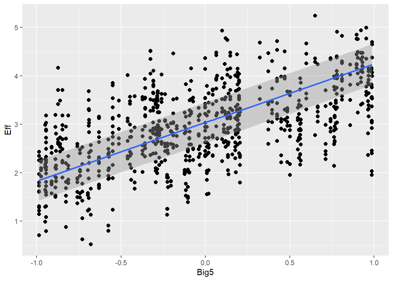
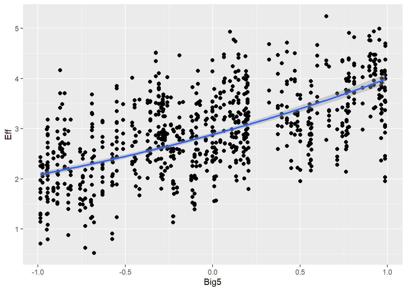
Personality traits (measured with Big5) will influence effort (e.g., people are more willing to put more effort if they are open-minded) and also communicative attempt (e.g., more extroverted people are better in this game, therefore they need less attempts)
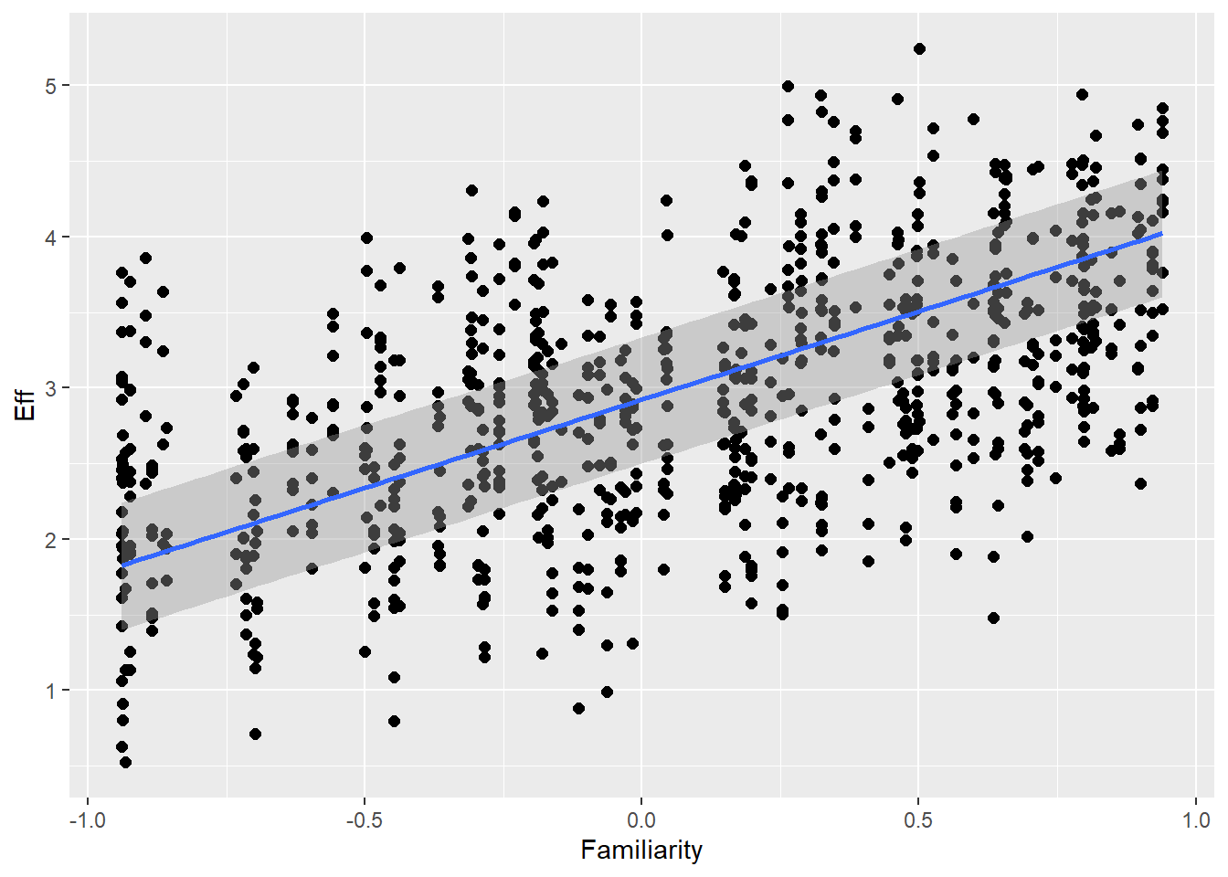
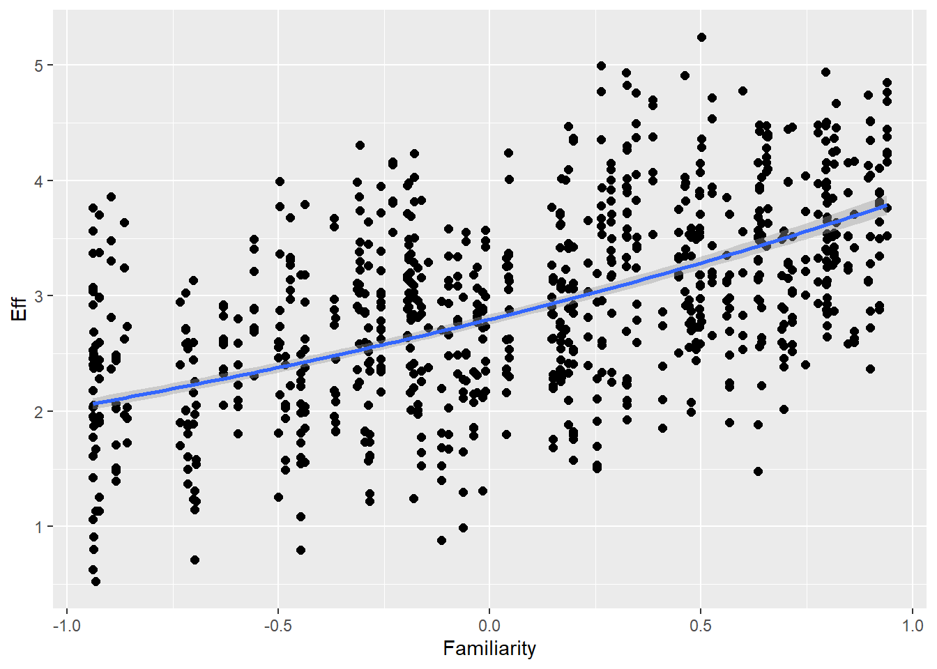
Familiarity with guessing partner influences effort (ditto) as well as communicative attempt (e.g., friends are better in this game than strangers)
Similarly, participant will also directly influence effort and commAtt, because personality traits might not be capturing all variation
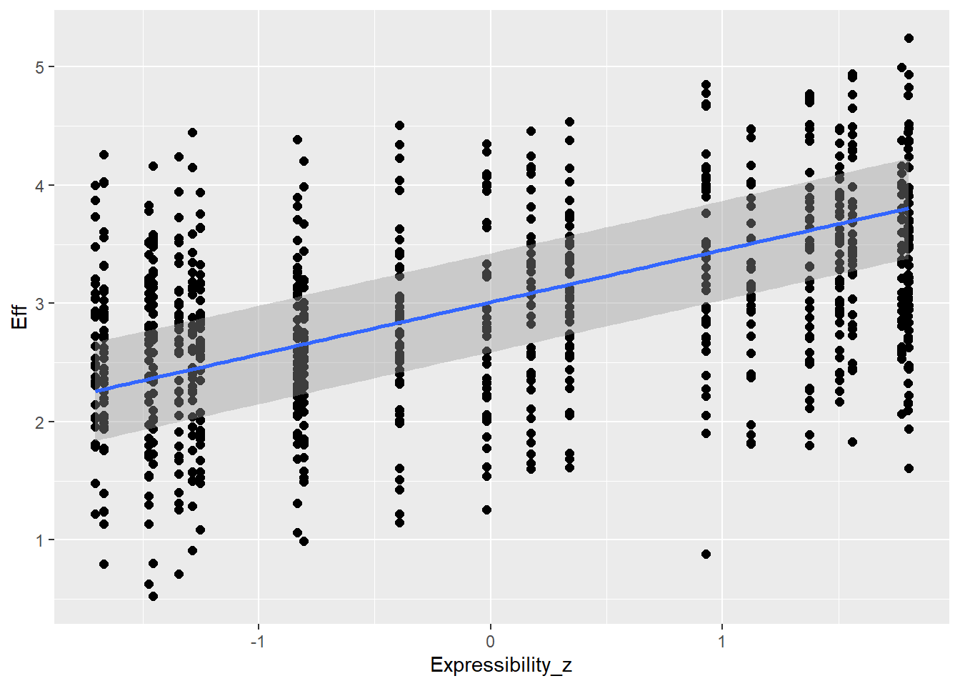
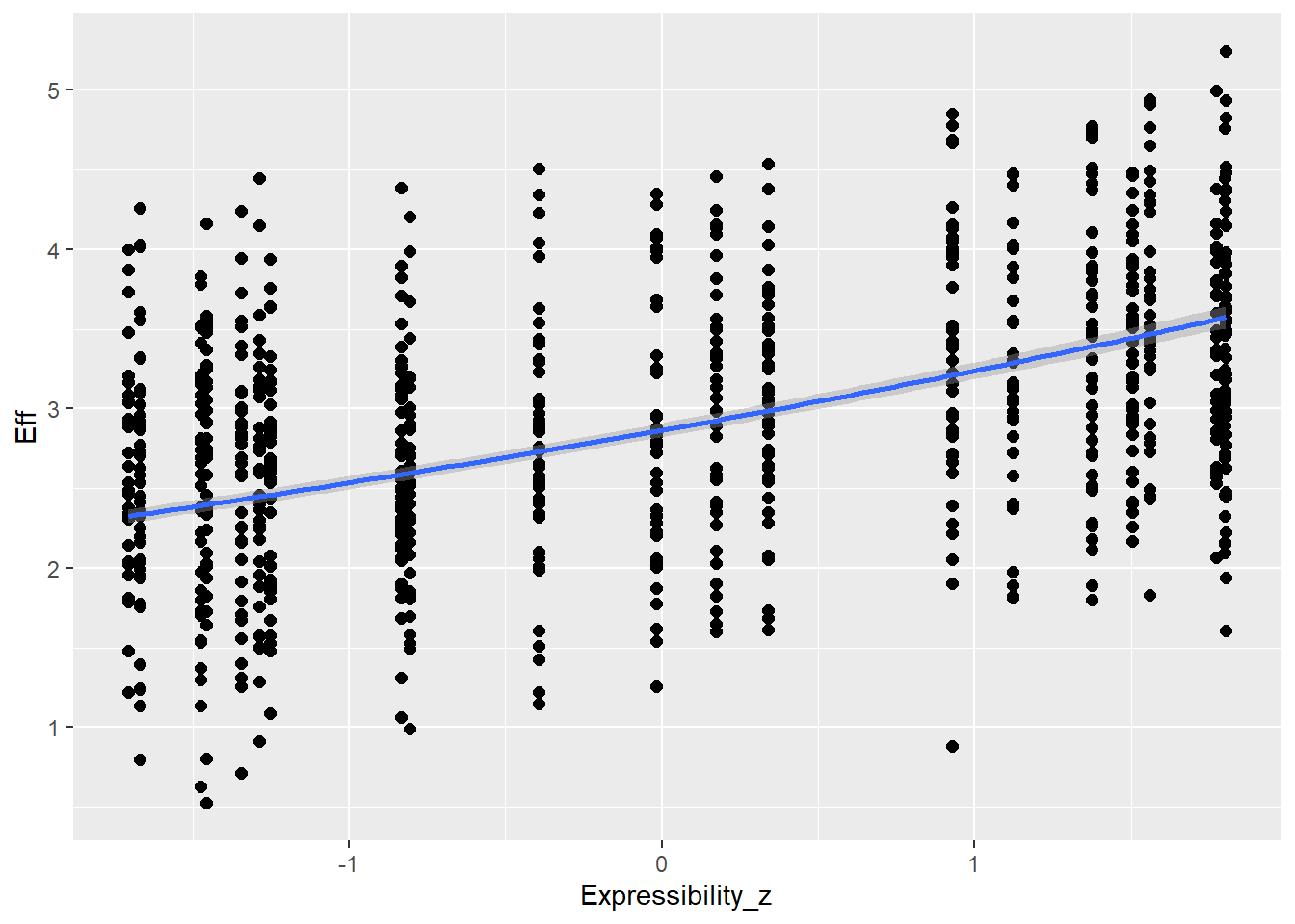
Expressibility of concepts is going to influence effort (e.g., more expressible concepts allow more enhancement - but could be also other direction) as well as CommAtt (e.g., more expressible concepts are more readily guessed and don’t need more attempts)
Similarly, concept will also directly influence effort and commAtt, because expressibility might not be capturing all variation
Modality (uni vs. multi) will influence the value of effort. We assume that in unimodal condition, the feature does not need to account for synergic relations with the other modality, and may carry the whole signal. In multimodal condition, however, there may be synergic relations that moderate the full expressiveness of this feature
Trial number (characterising how far one is in the experiment) could be hinting on learning processes through out the experiment, or - the other direction - on increasing fatigue
Note that we are aware that some of the parameters might be correlated and we might run into issues with collinearity. While DAG does not help to solve it, it does help in detecting whether the two potentially highly correlated variables have separate causal effect or share a common cause. If they share common cause, there might be a problem in distinguishing their effects from each other. We will report inter-variable correlations when analyzing the actual data.
These are the implied conditional independencies
Big5 _||_ Conc
Big5 _||_ Expr
Big5 _||_ Fam | Pcn
Big5 _||_ Mod
Big5 _||_ TrNm
Conc _||_ Fam
Conc _||_ Mod
Conc _||_ Pcn
Conc _||_ TrNm
Expr _||_ Fam
Expr _||_ Mod
Expr _||_ Pcn
Expr _||_ TrNm
Fam _||_ Mod
Fam _||_ TrNm
Mod _||_ Pcn
Mod _||_ TrNm
Pcn _||_ TrNm
This is the adjustment set that needs to be included in the model to make sure we are not confounding
{ Big5, Conc, Expr, Fam, Mod, Pcn, TrNum }
Creating synthetic data (for pre-registration purposes only)
Now we can proceed with creating synthetic data, incorporating the relationships we have acknowledged in our causal model. We will then use these data to validate the statistical models. We believe this approach constitutes a principled and transparent method for model validation (McElreath 2018; Morris, White, and Crowther 2019). By evaluating the model structure on simulated data before fitting it to empirical observations, we reduce the risk of overfitting and p-hacking, as model assumptions and inferences are tested independently of the observed data.
Note that the synthetic data do not copy the structure of the data and the experimental design perfectly, but they do provide a reliable ground to build the models and test their performance.
# Set seed for reproducibilityset.seed(0209)# Set coefficientsb_exp_vocal <-0.6# Vocal has lower expressibilityb_exp_multi <-1.5# Multimodal has higher expressibilityb_bif <-1.15# More extroverted → more effortb_fam <-1.10# More familiarity → more effortb_exp <-1.20# More expressibility → more effortb_multi <-0.70# Multimodal → slightly reduced effortb_comatt2 <-1.50# Effort increases for second attemptb_comatt3 <-0.50# Effort decreases for third attemptb_prevan <-0.50# Higher previous answer similarity → less effort# Define participants and conceptsn_participants <-120n_total_concepts <-21# Each participant works with all 21 conceptsn_modalities <-3# Gesture, vocal, combined# Generate participant-level dataparticipants <-1:n_participantsBig5 <-runif(n_participants, min =0, max =2)Familiarity <-runif(n_participants, min =0, max =2)# Generate expressibility scores for each concept across modalitiesexpressibility_matrix <-matrix(runif(n_total_concepts * n_modalities, min =0, max =1),nrow = n_total_concepts, ncol = n_modalities)# Initialize data storagefinal_data_synt <-data.frame()# Define function to simulate participant datasimulate_participant <-function(participant_id) { participant_data <-data.frame() trial_number <-1for (concept_id in1:n_total_concepts) {# Assign a random modality modality <-sample(c("gesture", "vocal", "combined"), 1)# Get expressibility score based on modality expressibility_score <-ifelse(modality =="vocal", expressibility_matrix[concept_id, 1] * b_exp_vocal, ifelse(modality =="gesture", expressibility_matrix[concept_id, 2], expressibility_matrix[concept_id, 3] * b_exp_multi))# Base effort before adjustments base_effort <- b_bif * Big5[participant_id] + b_fam * Familiarity[participant_id] + b_exp * expressibility_score +rnorm(1, mean =1, sd =0.5)# Adjust effort for multimodal conditionif (modality =="combined") { base_effort <- base_effort * b_multi }# Sample the number of communicative attempts (CommAtt) adjusted_prob <-c(1- Familiarity[participant_id],1- Familiarity[participant_id],1- Familiarity[participant_id]) *c(1- Big5[participant_id],1- Big5[participant_id],1- Big5[participant_id]) *c(1- expressibility_score,1- expressibility_score,1- expressibility_score) adjusted_prob <- adjusted_prob /sum(adjusted_prob) n_attempts <-sample(1:3, 1, prob = adjusted_prob) prev_answer_similarity <-NA# First attempt has no previous similarity# Generate rows for each communicative attemptfor (attempt in1:n_attempts) { Eff <- base_effort # Start with base effort# Modify effort for second and third attemptsif (attempt ==2) { Eff <- Eff * b_comatt2 } elseif (attempt ==3) { Eff <- Eff * b_comatt3 }# Adjust effort based on previous answer similarityif (!is.na(prev_answer_similarity)) { Eff <- Eff * (1+ (1- prev_answer_similarity) * b_prevan) }# Store row participant_data <-rbind(participant_data, data.frame(Participant = participant_id,Concept = concept_id,Modality = modality,Big5 = Big5[participant_id],Familiarity = Familiarity[participant_id],Expressibility = expressibility_score,CommAtt = attempt,Eff = Eff,TrialNumber = trial_number,PrevAn = prev_answer_similarity ))# Update for next attempt trial_number <- trial_number +1 prev_answer_similarity <-runif(1, min =0, max =1) # Simulate next similarity } }return(participant_data)}# Simulate data for all participantsfinal_data_synt <-do.call(rbind, lapply(participants, simulate_participant))# Preview resultshead(final_data_synt, n=15)
final_data$TrialNumber_c <- final_data$TrialNumber -median(range(final_data$TrialNumber))final_data$Familiarity <- final_data$Familiarity -median(range(final_data$Familiarity))final_data$Big5 <- final_data$Big5 -median(range(final_data$Big5))# For now, we will just center Familiarity and Big5 because we created them synthetically. But the real data have these two variables already z-scored
First we want to do a simple model that reproduce our DAG.
Our main predictor is communicative attempt (CommAtt). To account for confounders - variables affecting both the predictor and the dependent variable - we need to adjust for them in the model by including them as covariates to isolate the effect of the predictor. Based on our DAG, confounders include:
familiarity
big5
expressibility
trial number
modality
concept
participant
We include 1.-5. as fixed factors. For 6.-7., we include varying intercepts as we expect that each participant and concept may have they own baseline level of effort and thus allow for individual variation. Partial pooling is also beneficial in that extreme values (or categories will fewer datapoints) will be shrunk toward the overal average.
We will now not include PrevAn (previous answer) variable because we will need to do some further data-wrangling when building model for H2. That is mainly because PrevAn has some NA values, concretely for first attempts. Models would automatically exclude NA data, and we would therefore loose all effort data for attempt 1. For H1, however, we want to keep it there.
This is our first model without setting any priors, leaving them to default values
h1.m1 <-brm(Eff ~1+ CommAtt + Familiarity + Big5 + Expressibility_z + TrialNumber_c + Modality + (1| Participant) + (1| Concept),data = final_data,iter =4000,cores =4)# Add criterions for later diagnosticsh1.m1 <-add_criterion(h1.m1, criterion =c("loo", "waic"))# Calculate also variance explained (R^2)h1.m1_R2 <-bayes_R2(h1.m1)# Save both as objectssaveRDS(h1.m1, here("09_Analysis_Modeling", "models", "h1.m1.rds"))saveRDS(h1.m1_R2, here("09_Analysis_Modeling", "models", "h1.m1_R2.rds"))beep(5)
Family: gaussian
Links: mu = identity; sigma = identity
Formula: Eff ~ 1 + CommAtt + Familiarity + Big5 + Expressibility_z + TrialNumber_c + Modality + (1 | Participant) + (1 | Concept)
Data: final_data (Number of observations: 5076)
Draws: 4 chains, each with iter = 4000; warmup = 2000; thin = 1;
total post-warmup draws = 8000
Multilevel Hyperparameters:
~Concept (Number of levels: 21)
Estimate Est.Error l-95% CI u-95% CI Rhat Bulk_ESS Tail_ESS
sd(Intercept) 0.04 0.02 0.00 0.09 1.00 2122 1863
~Participant (Number of levels: 120)
Estimate Est.Error l-95% CI u-95% CI Rhat Bulk_ESS Tail_ESS
sd(Intercept) 0.03 0.02 0.00 0.07 1.00 2320 3475
Regression Coefficients:
Estimate Est.Error l-95% CI u-95% CI Rhat Bulk_ESS Tail_ESS
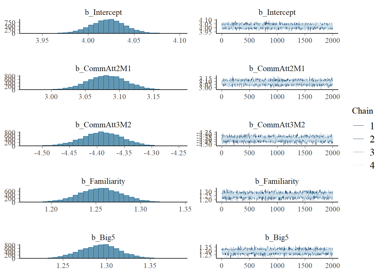
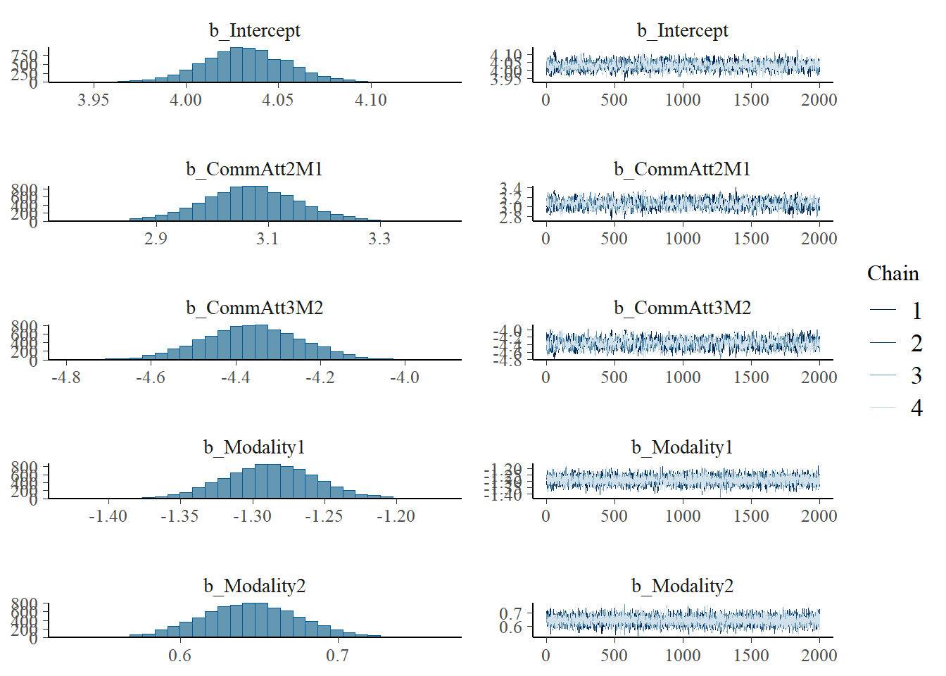
Intercept 4.02 0.02 3.98 4.06 1.00 6694 5622
CommAtt2M1 3.08 0.03 3.03 3.14 1.00 8963 6147
CommAtt3M2 -4.39 0.04 -4.46 -4.32 1.00 8289 5880
Familiarity 1.26 0.02 1.21 1.30 1.00 8380 5226
Big5 1.29 0.02 1.25 1.34 1.00 9979 6018
Expressibility_z 0.46 0.02 0.43 0.49 1.00 9888 5989
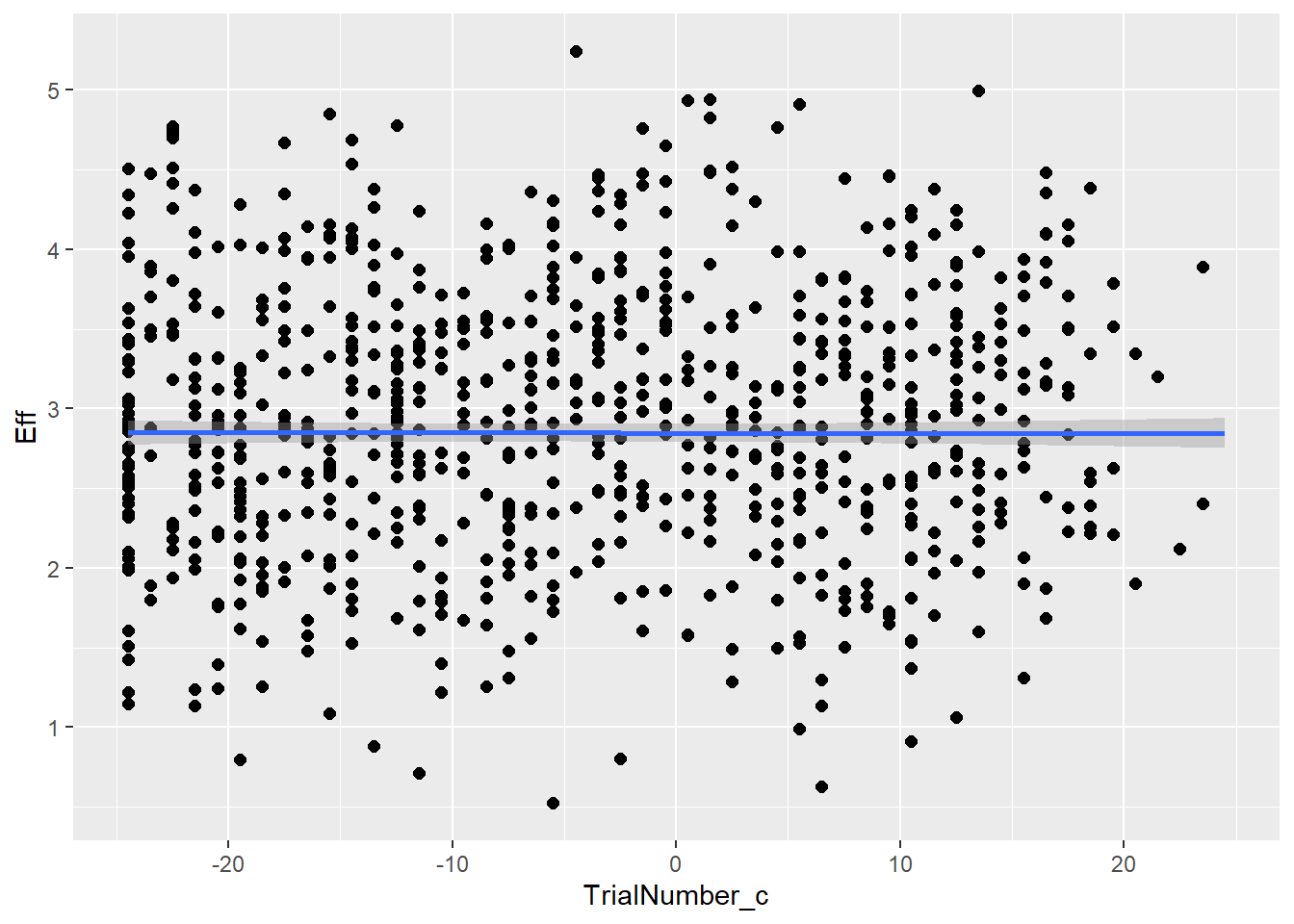
TrialNumber_c -0.00 0.00 -0.00 0.00 1.00 7595 5984
Modality1 -1.30 0.04 -1.38 -1.23 1.00 8559 5997
Modality2 0.64 0.04 0.57 0.71 1.00 7347 5787
Further Distributional Parameters:
Estimate Est.Error l-95% CI u-95% CI Rhat Bulk_ESS Tail_ESS
sigma 0.91 0.01 0.89 0.93 1.00 11791 5667
Draws were sampled using sampling(NUTS). For each parameter, Bulk_ESS
and Tail_ESS are effective sample size measures, and Rhat is the potential
scale reduction factor on split chains (at convergence, Rhat = 1).
Note
Note on modality: Modality1 represents the baseline difference between combined and the other modalities, and Modality2 represents the difference between gesture and vocal compared to combined.
Transforming coefficients
To be able to link these estimates back to the simulation coefficients, let’s create a function
transform_attempt <-function(intercept, CommAtt2M1, CommAtt3M2) {# Effort for the first attempt (base effort) Eff_attempt_1 <- intercept# Effort for the second attempt Eff_attempt_2 <- Eff_attempt_1 + CommAtt2M1# Effort for the third attempt Eff_attempt_3 <- Eff_attempt_1 + CommAtt2M1 + CommAtt3M2# Calculate ratios b_attempt2 <- Eff_attempt_2 / Eff_attempt_1 b_attempt3 <- Eff_attempt_3 / Eff_attempt_2return(data.frame(b_attempt2, b_attempt3))}h1m1_coeff <-transform_attempt(4.02, 3.08, -4.39)print(h1m1_coeff)
  b_attempt2 b_attempt3
1   1.766169  0.3816901
# For centered familiarityfam = (4.02+1.26) /4.02print(fam)
[1] 1.313433
# For centered BIFbif = (4.02+1.29) /4.02print(bif)
[1] 1.320896
Note
Expressibility is z-scored so we will not get to the coefficient in the same way but we can check the conditinal effects for checking whether it looks good
Let’s also check the visuals
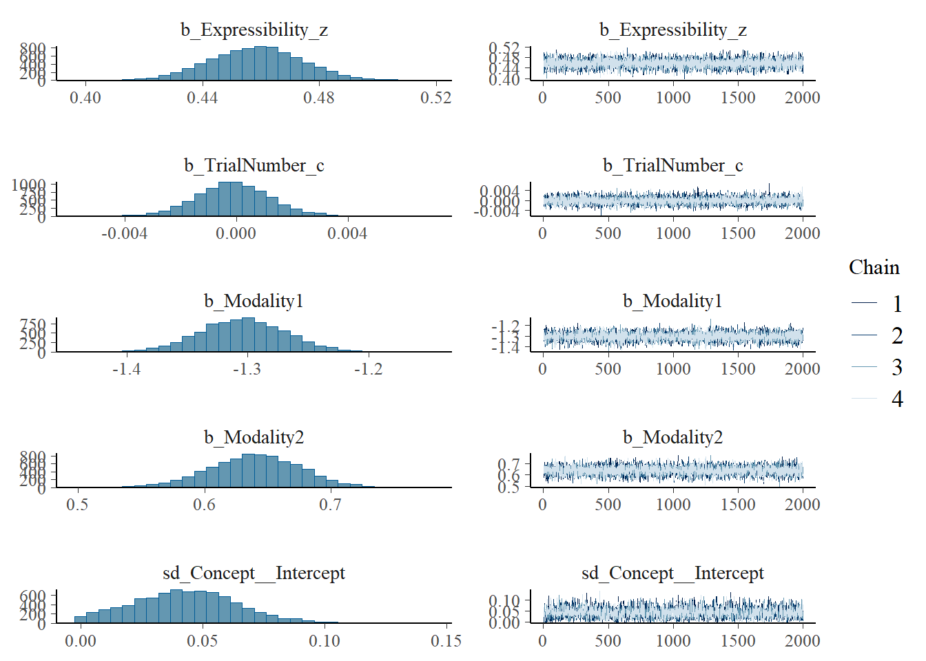
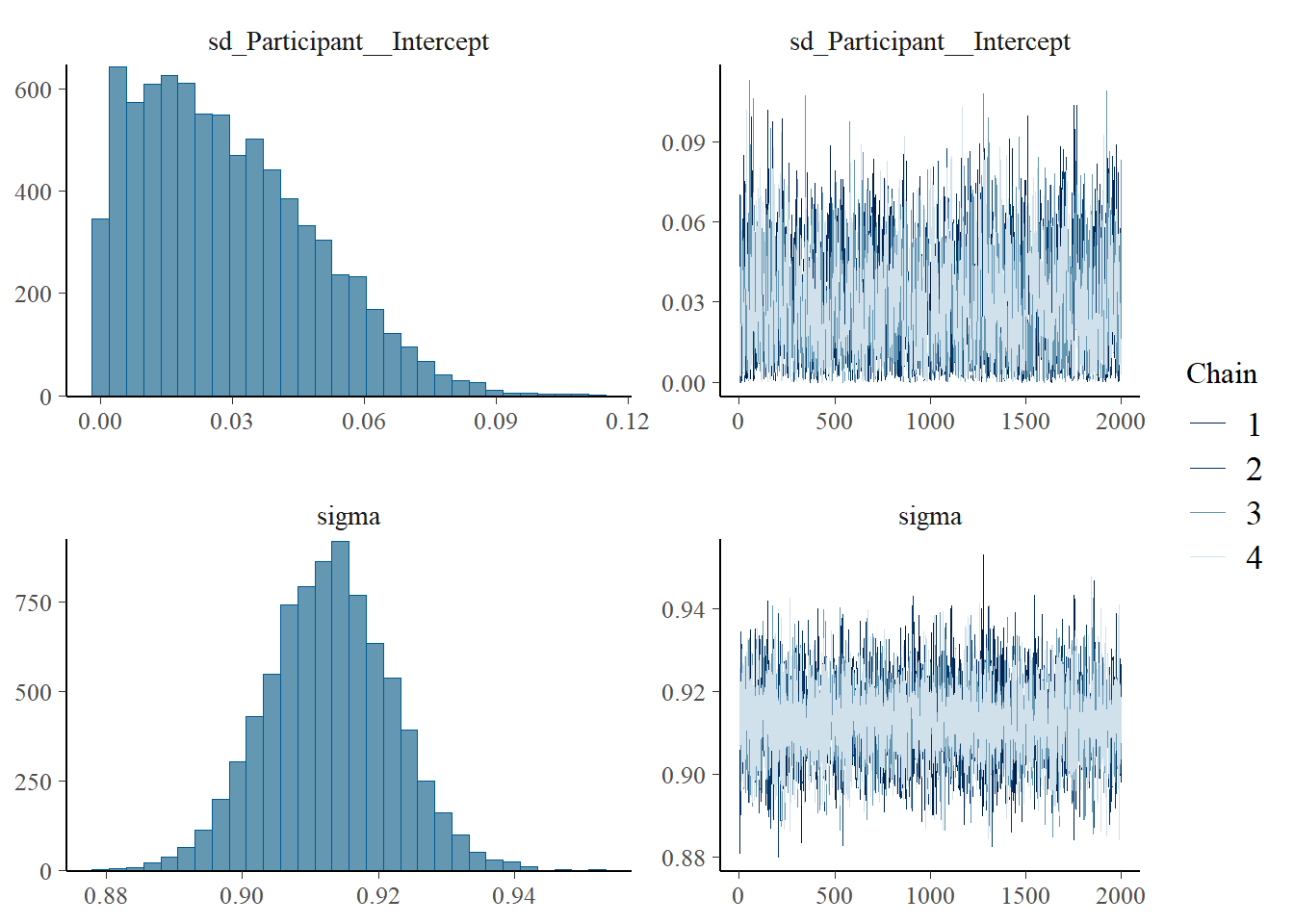
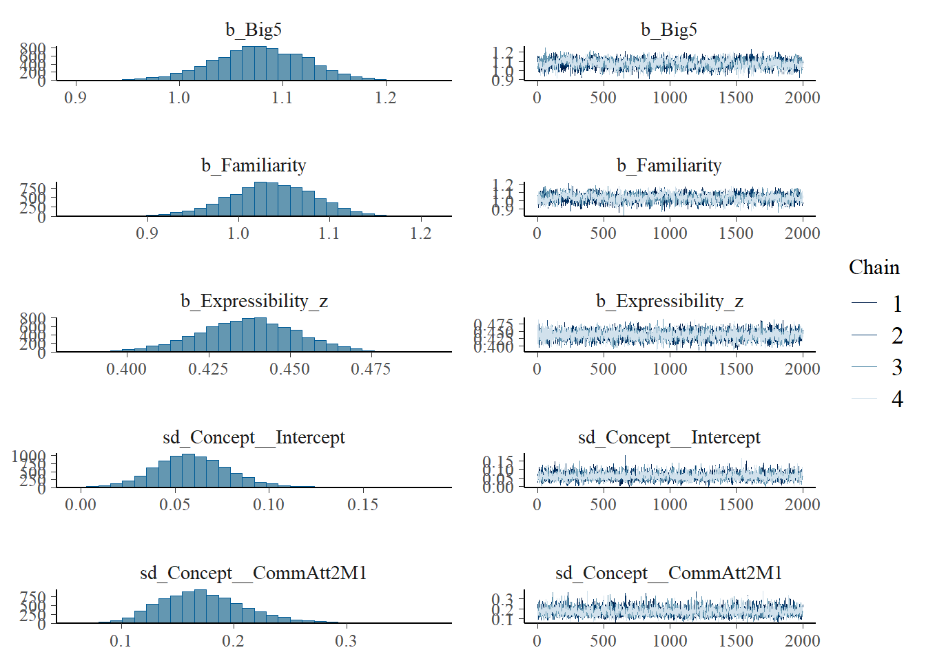
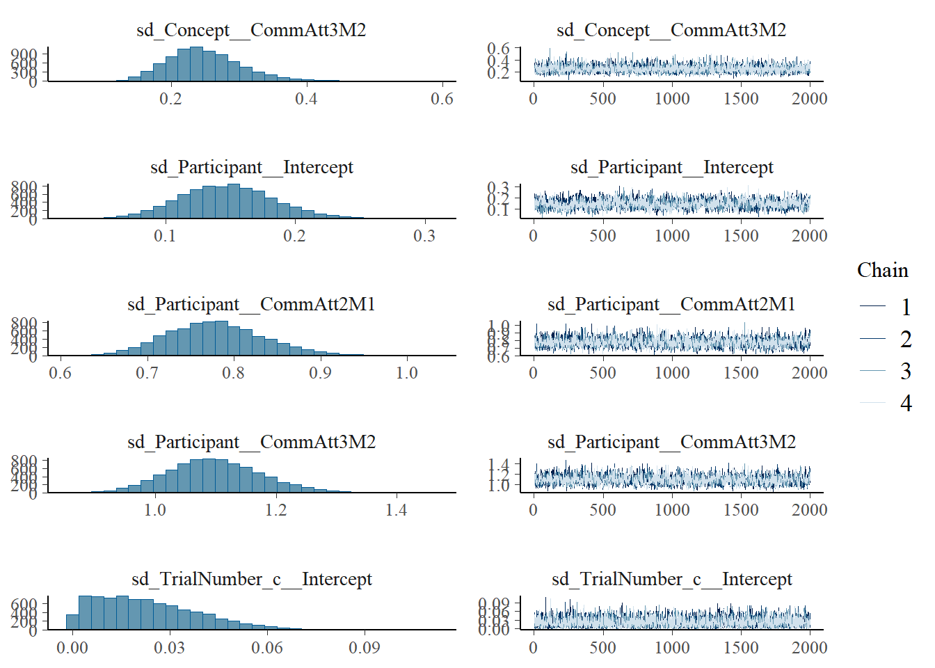
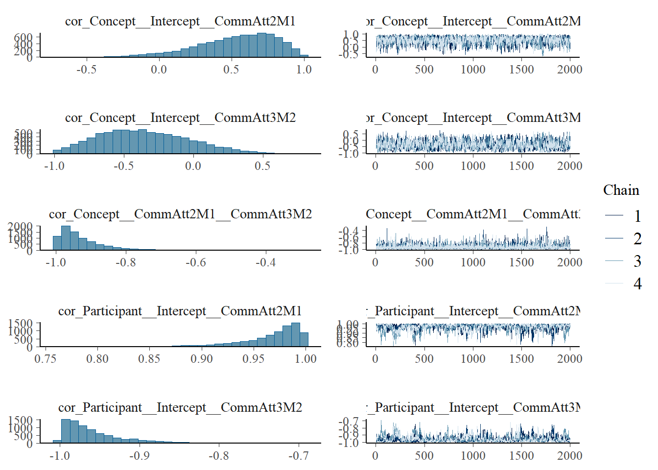
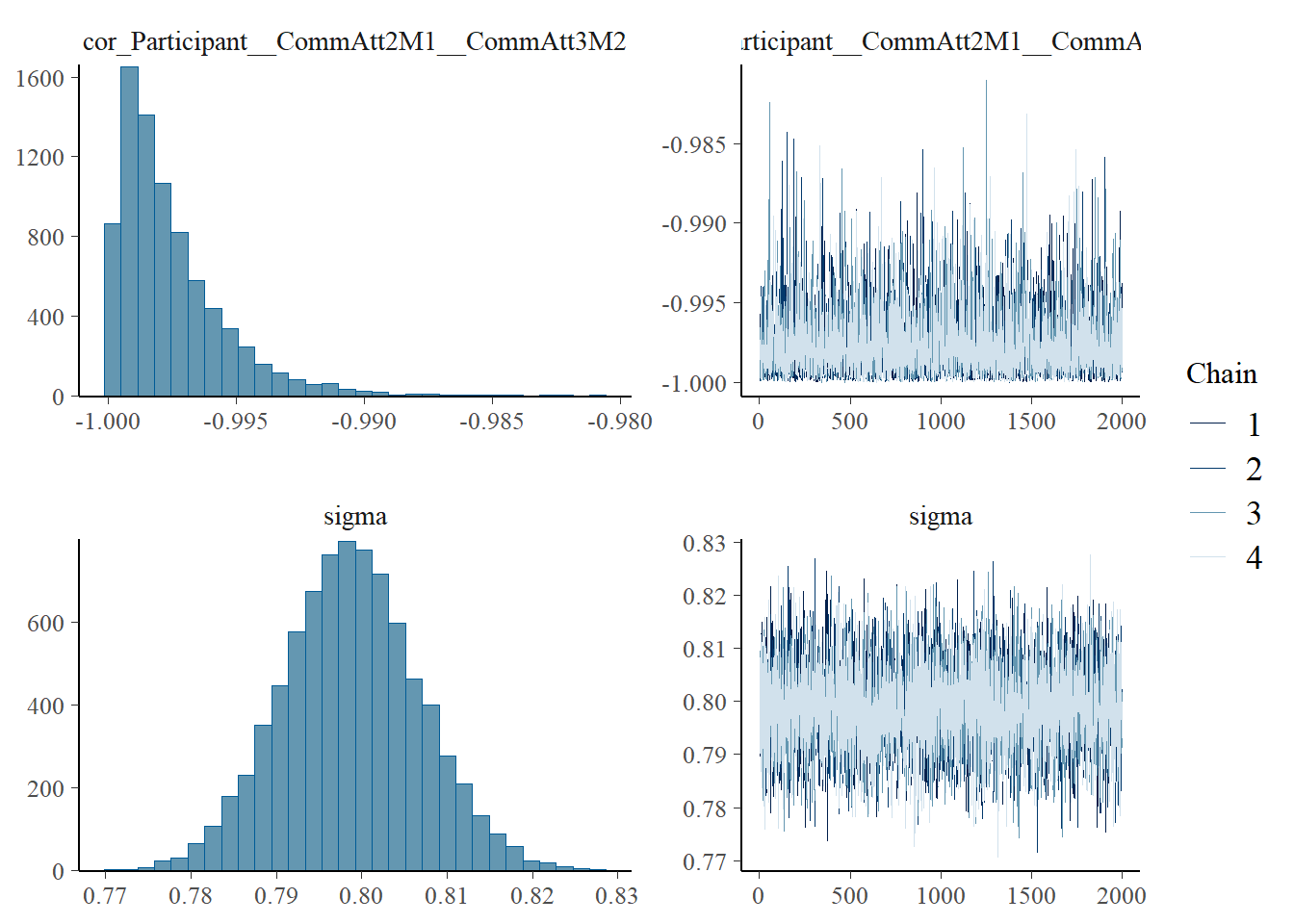
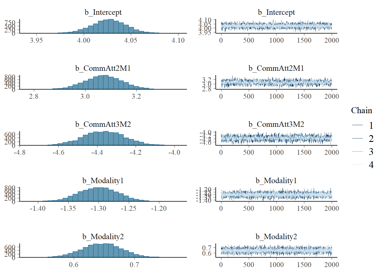
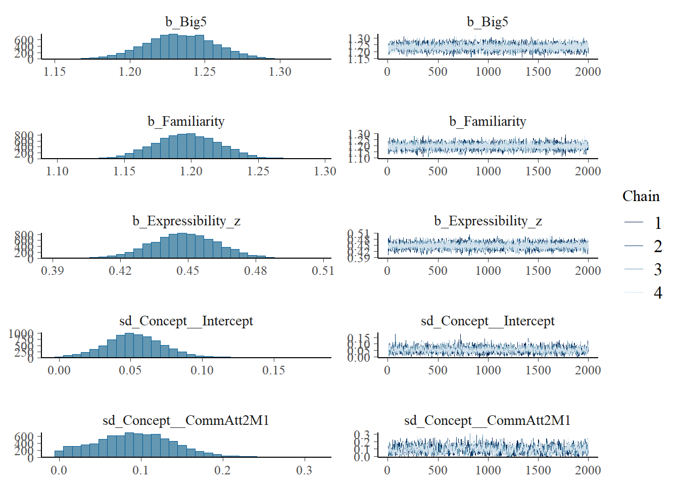
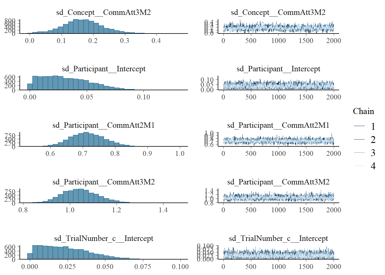
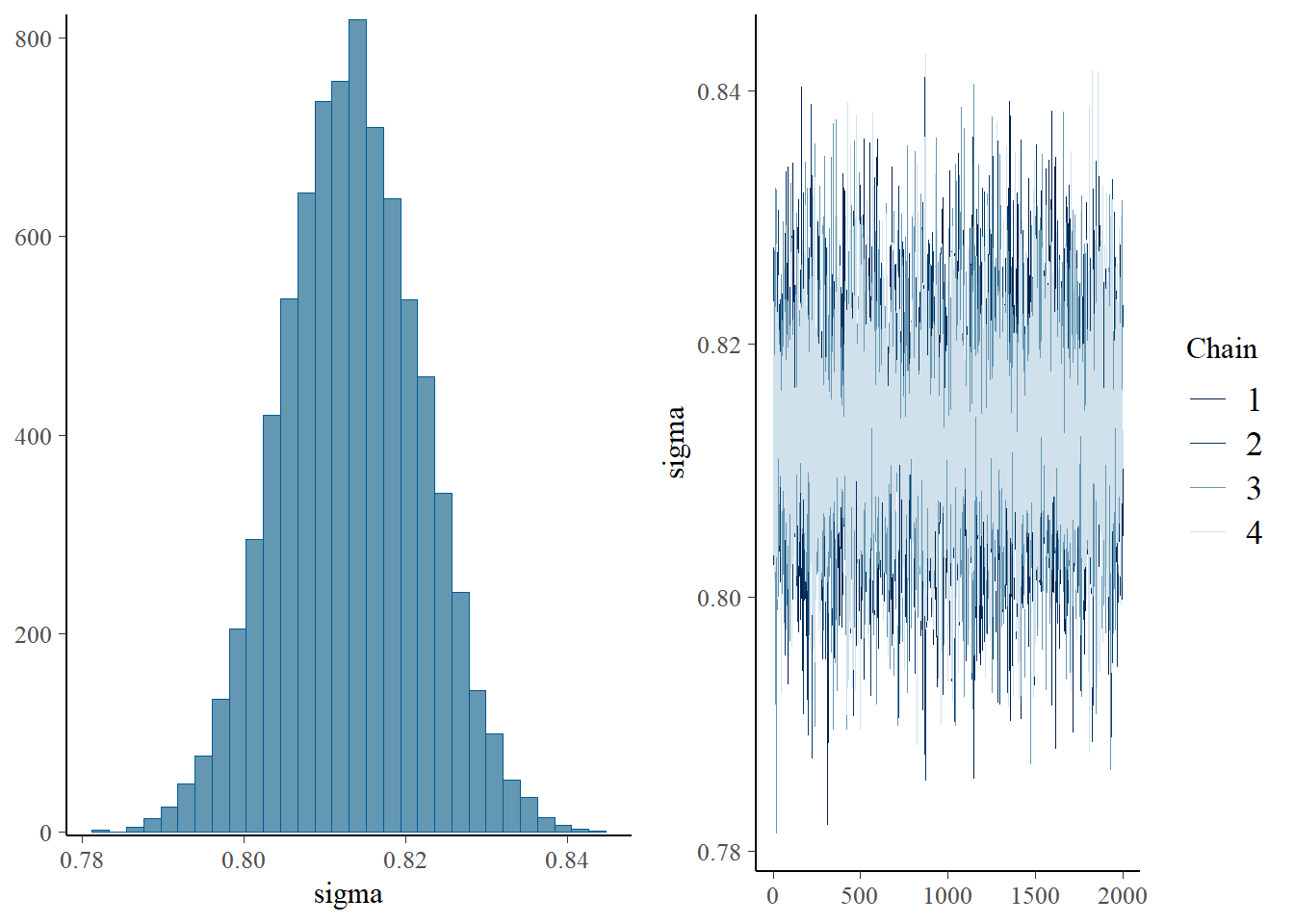
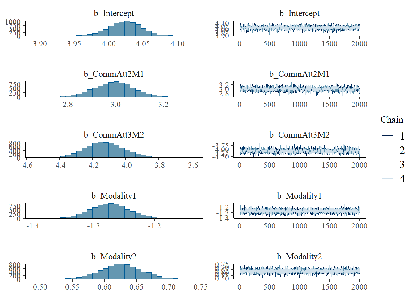
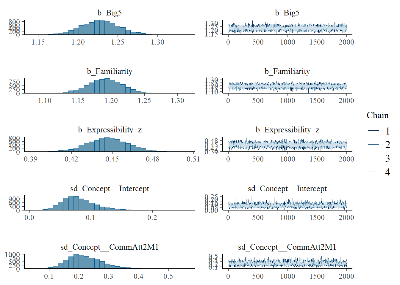
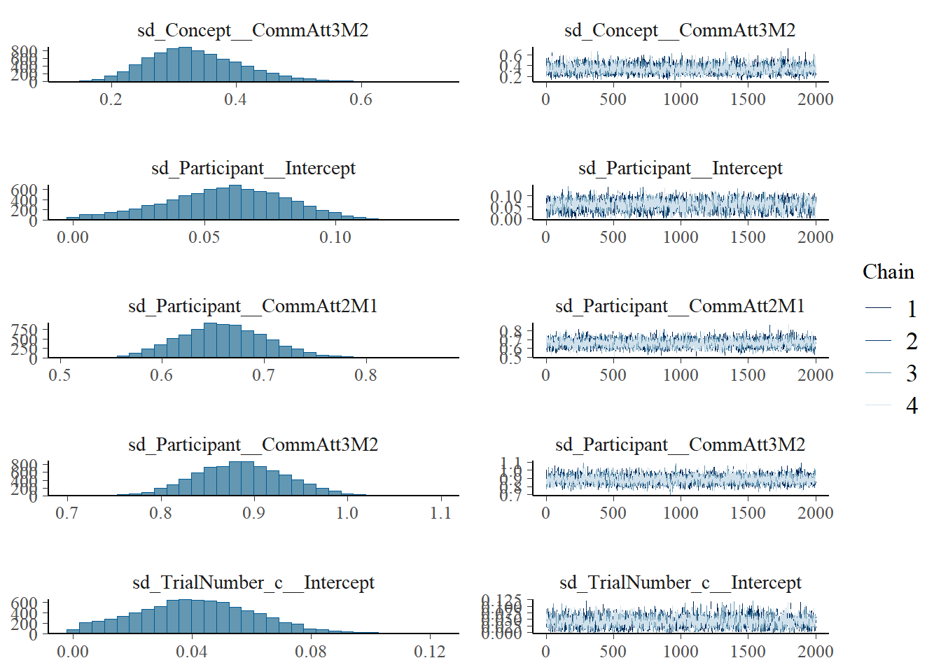
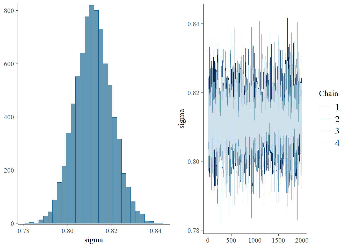
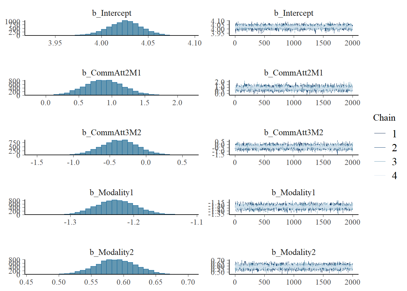
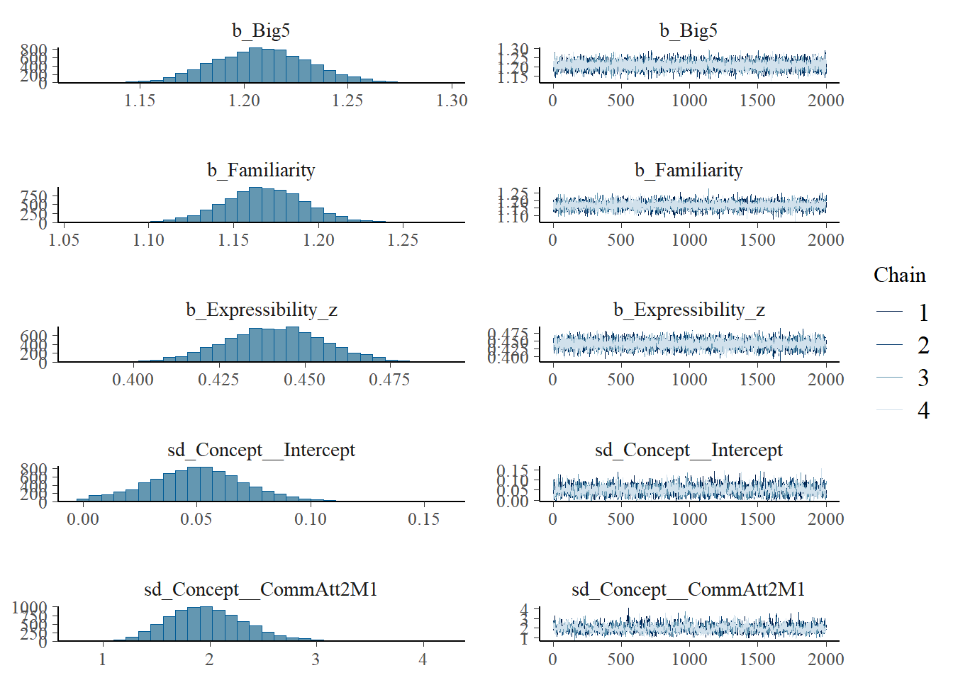
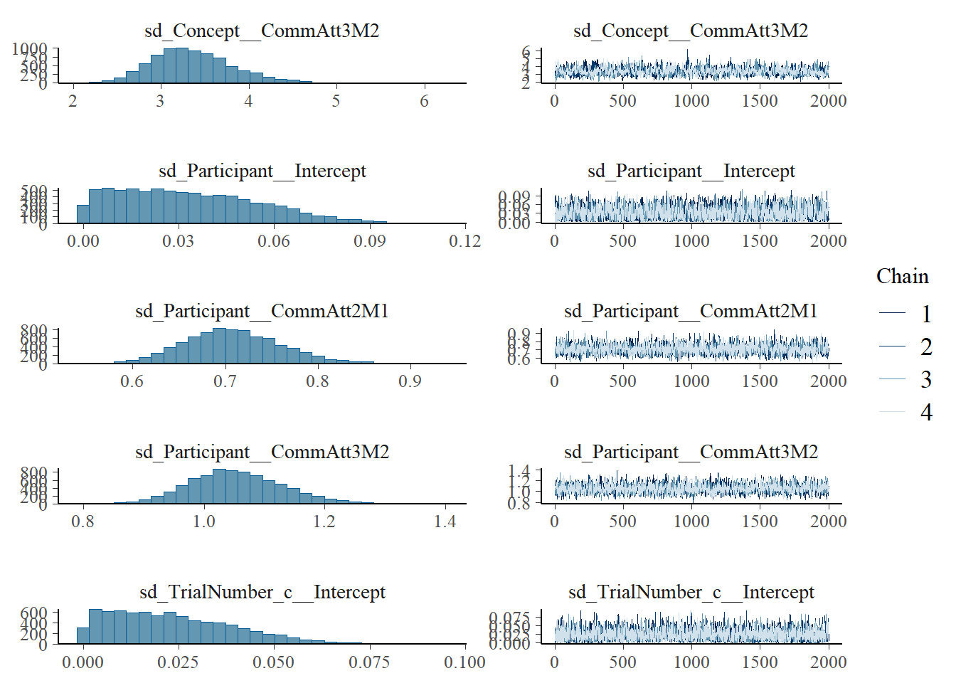
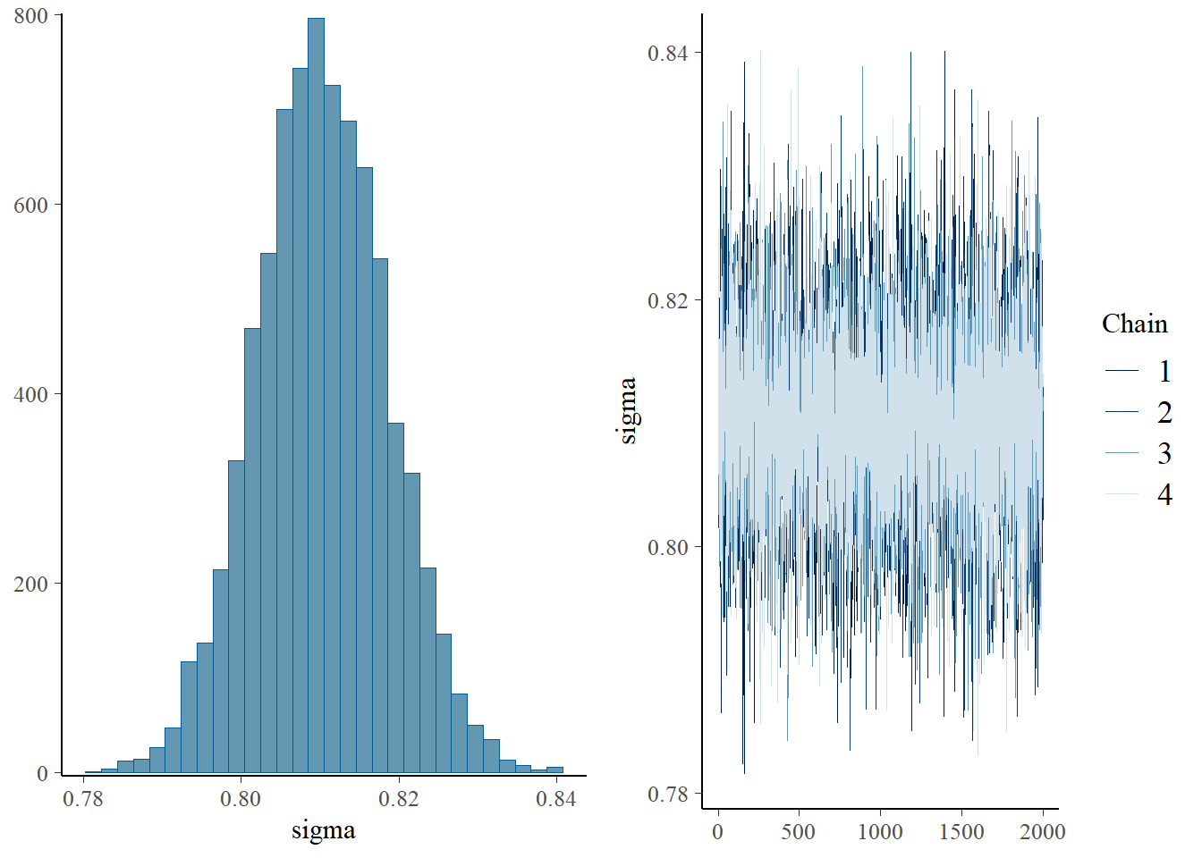
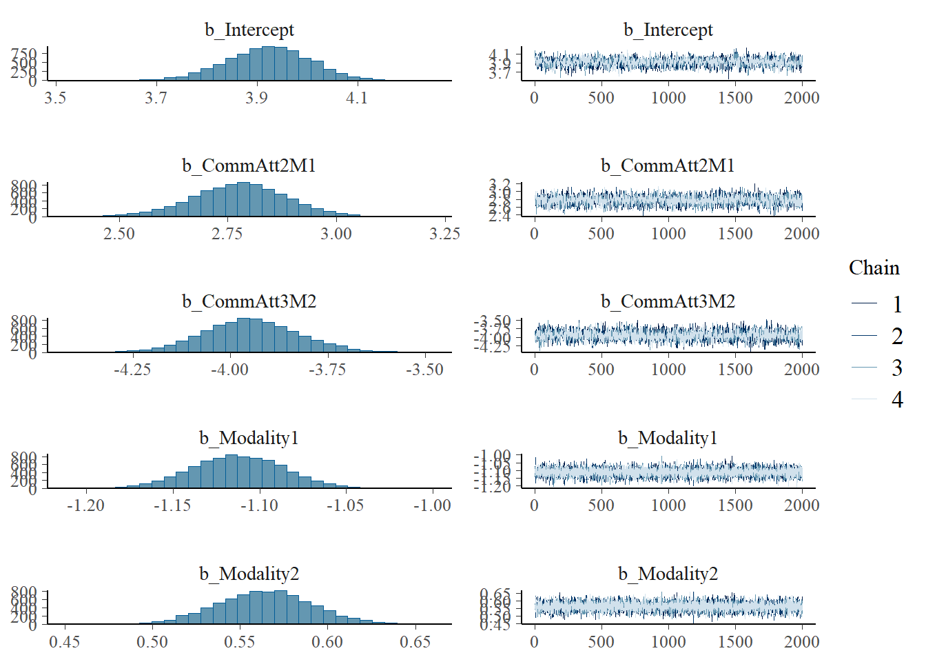
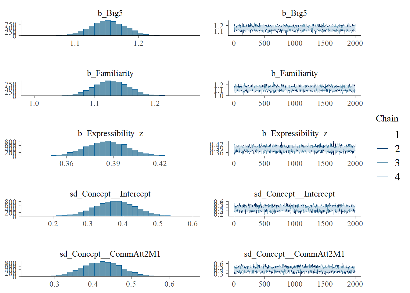
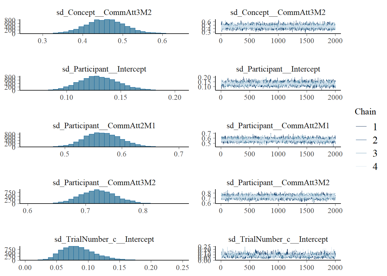
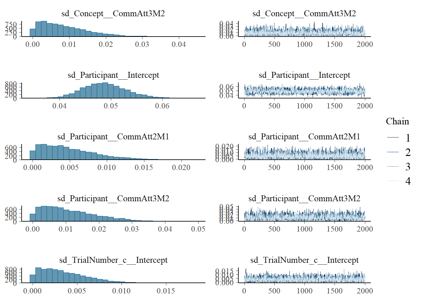
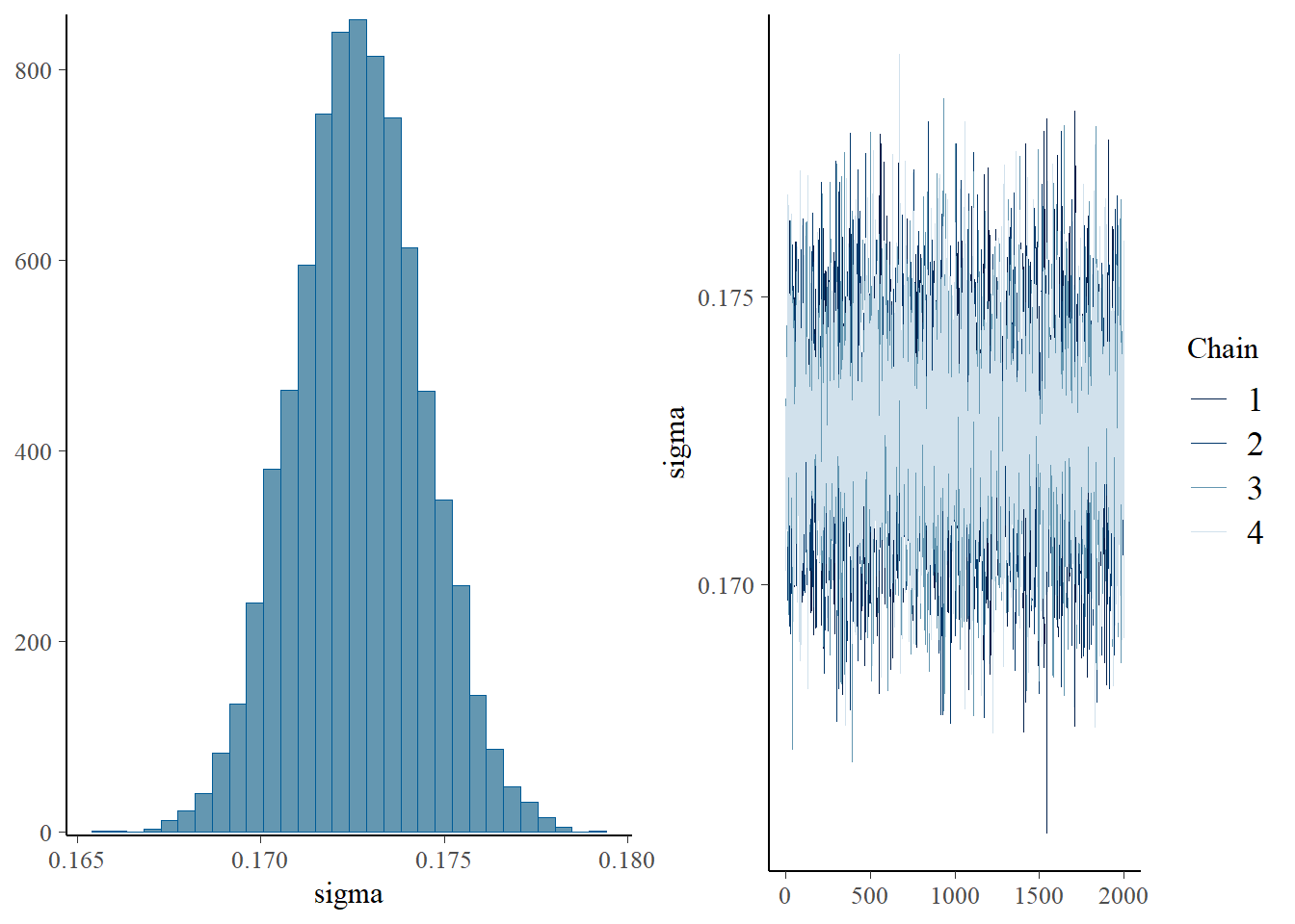
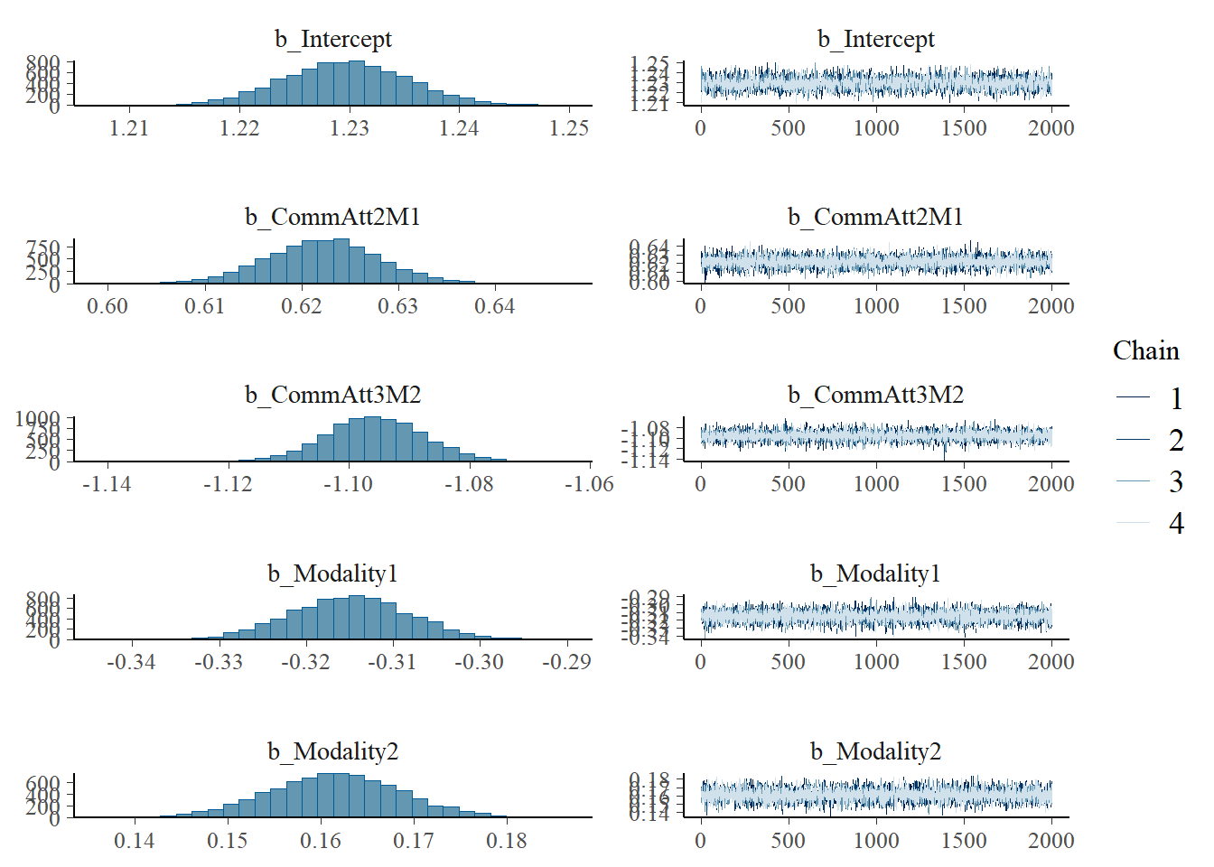
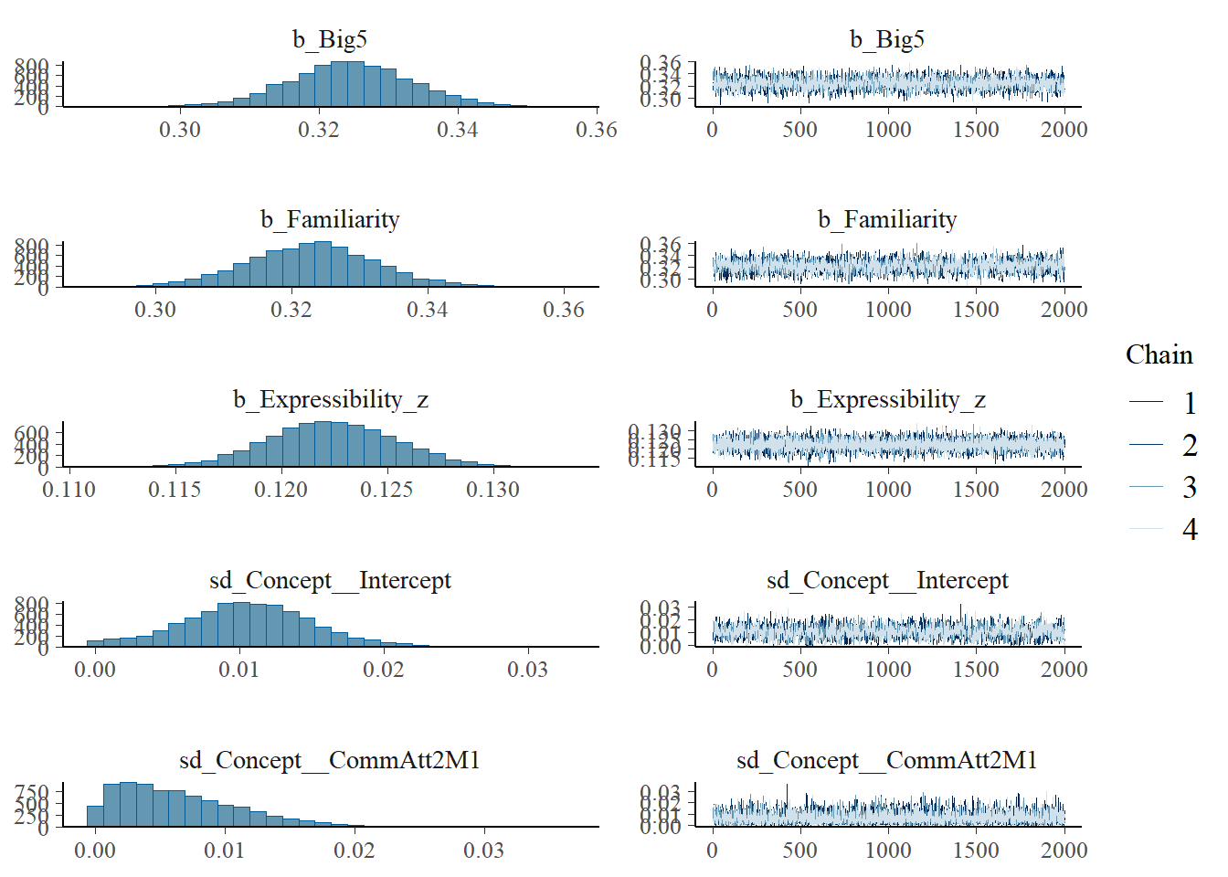
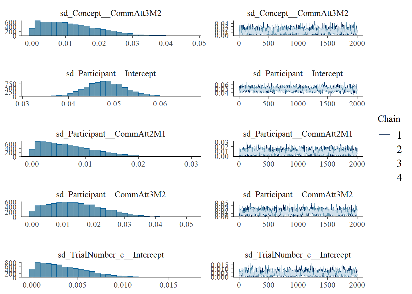
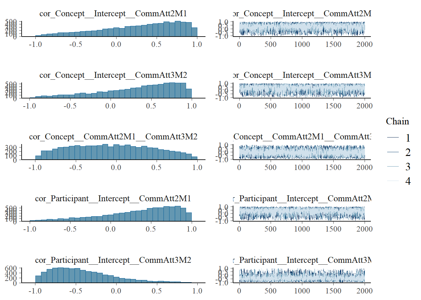
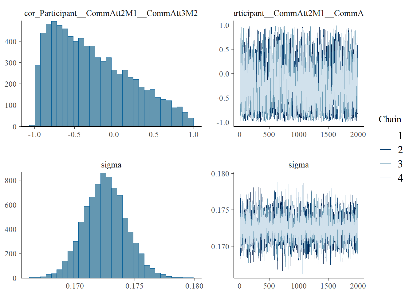
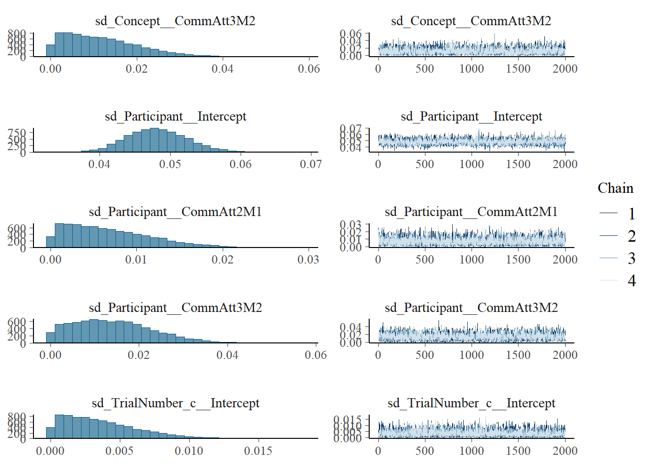
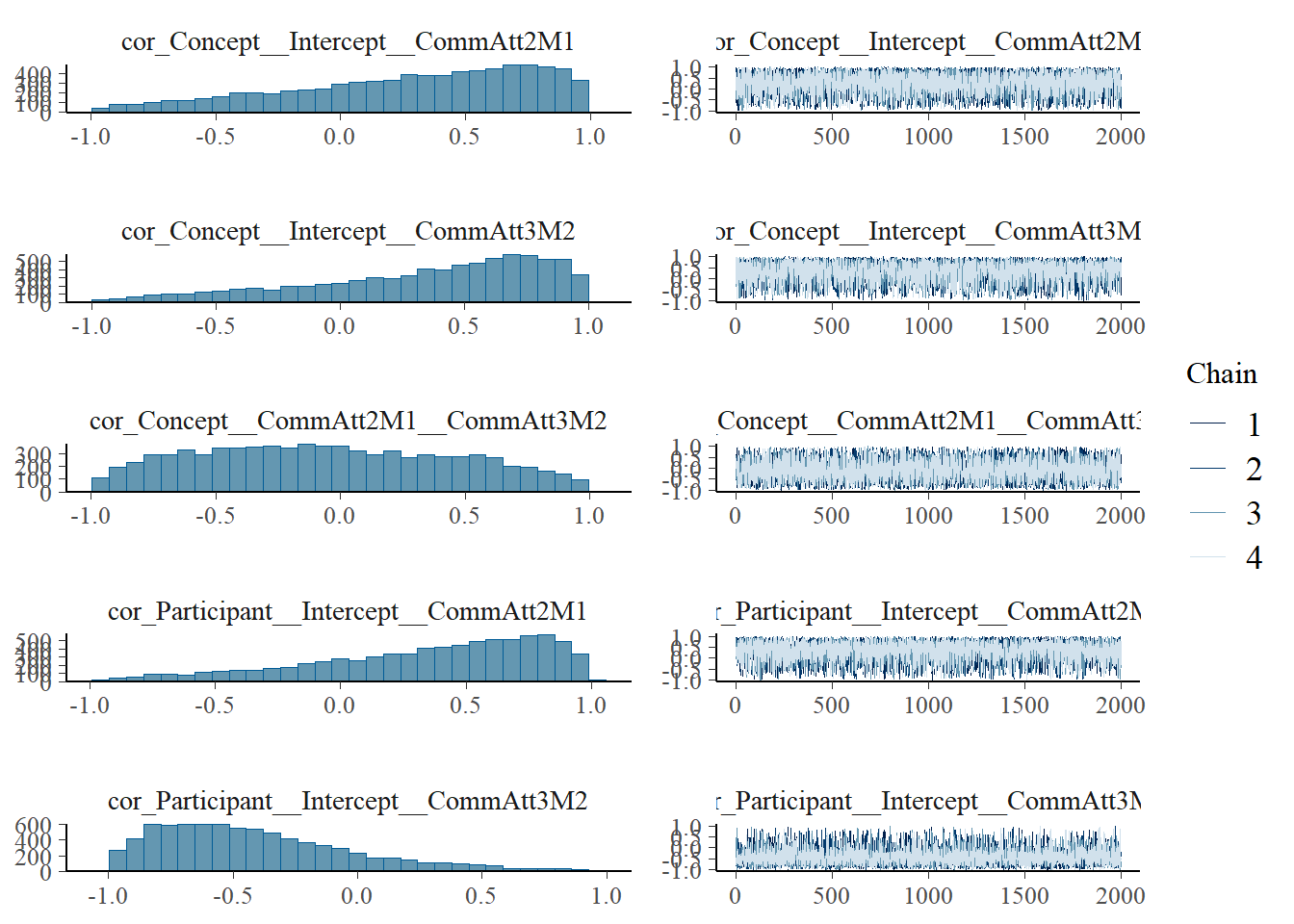
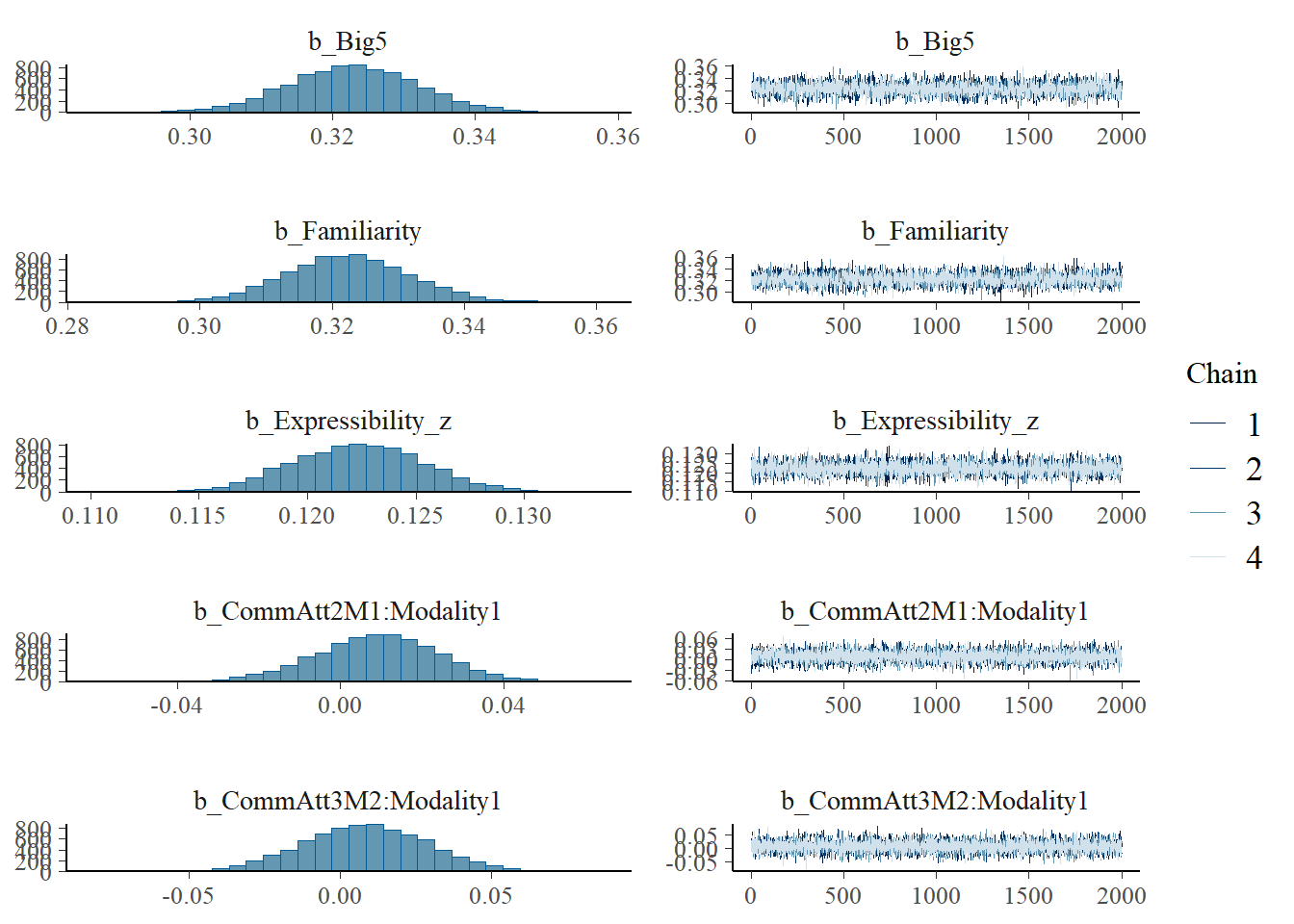
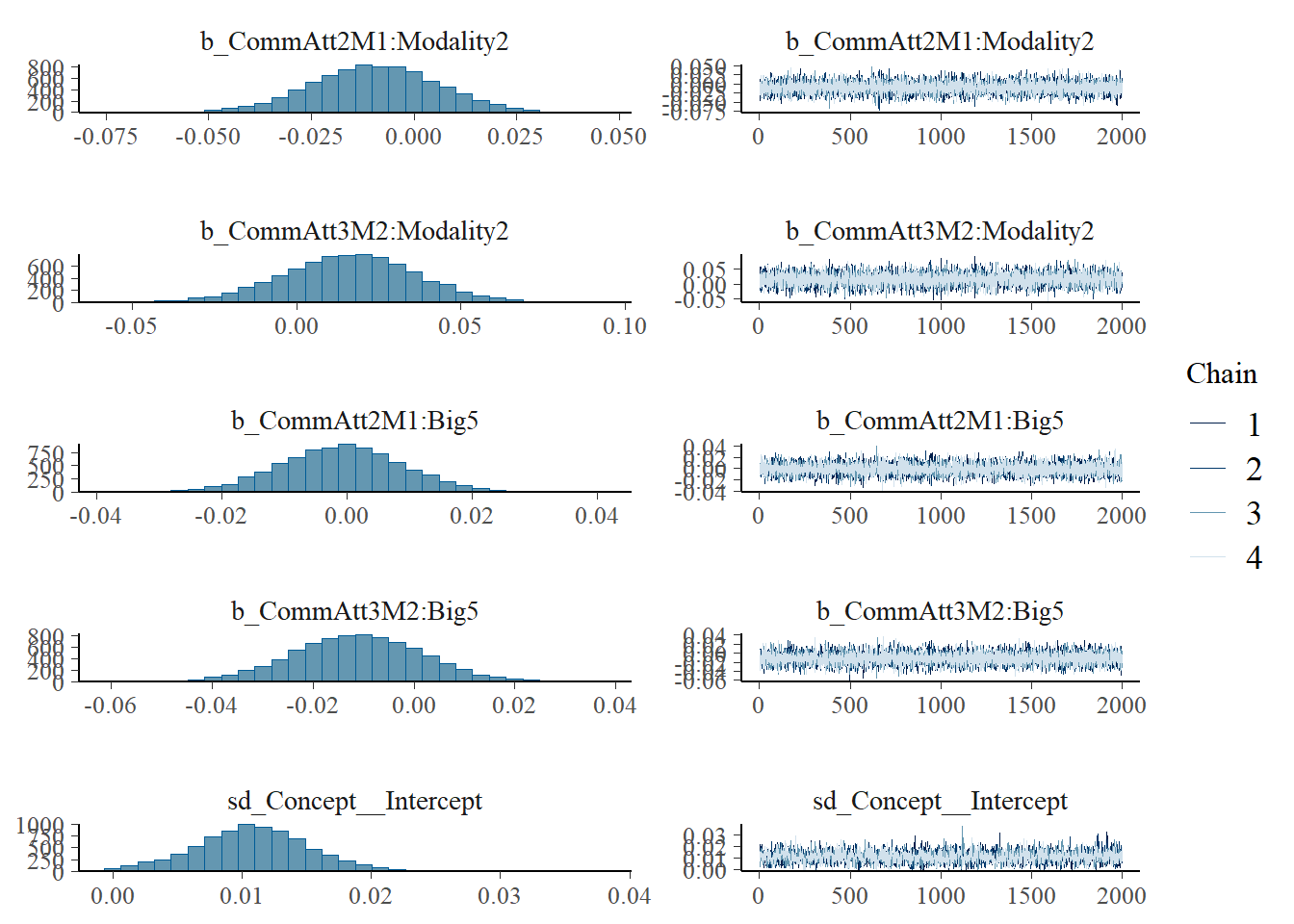
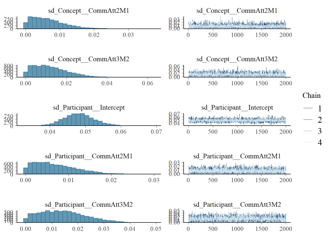
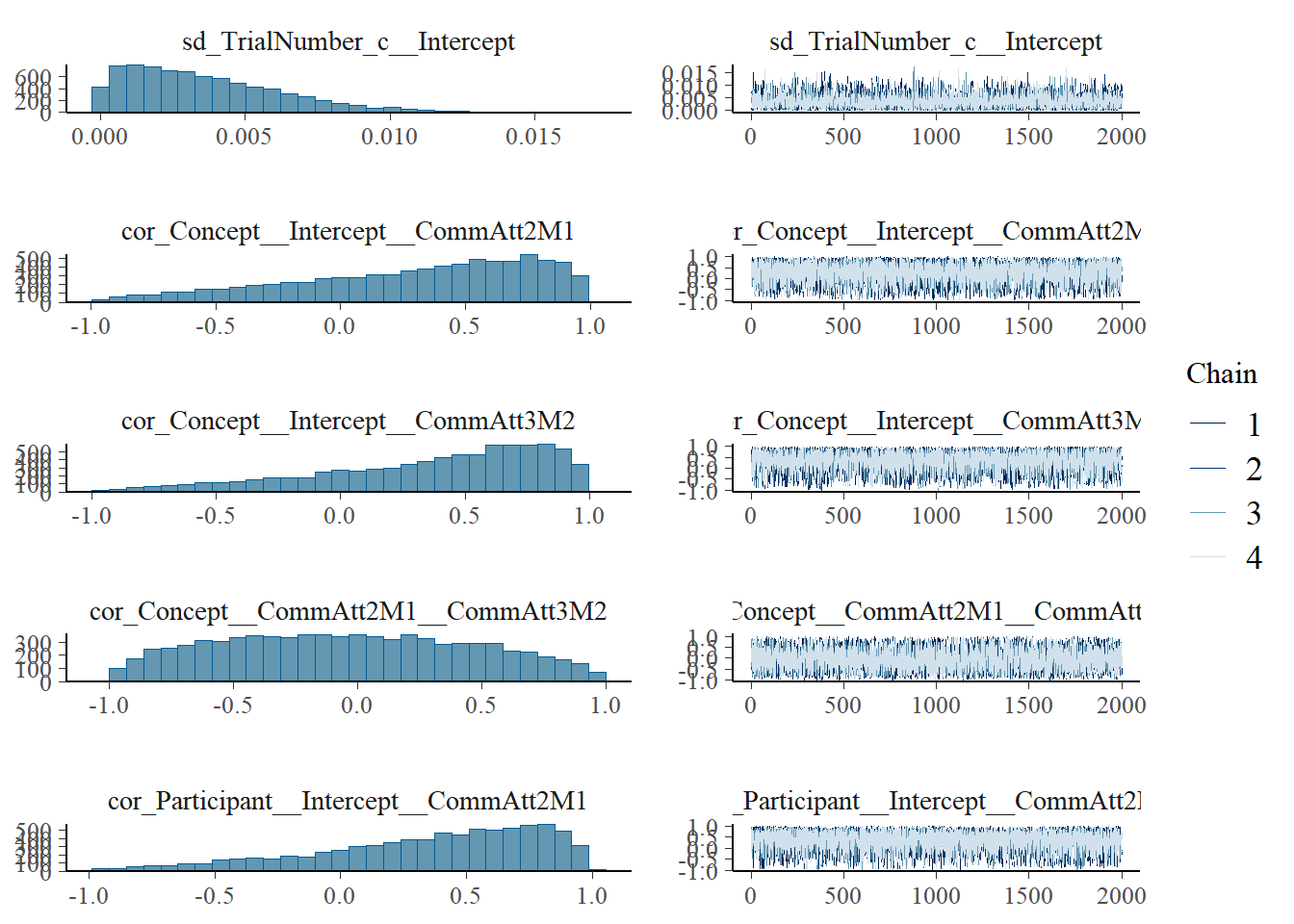
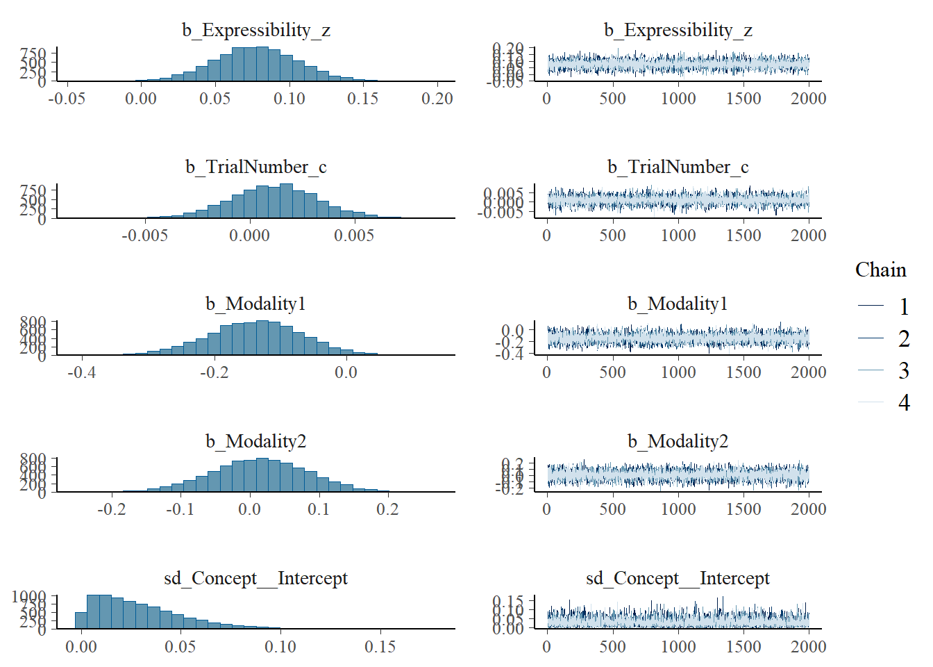
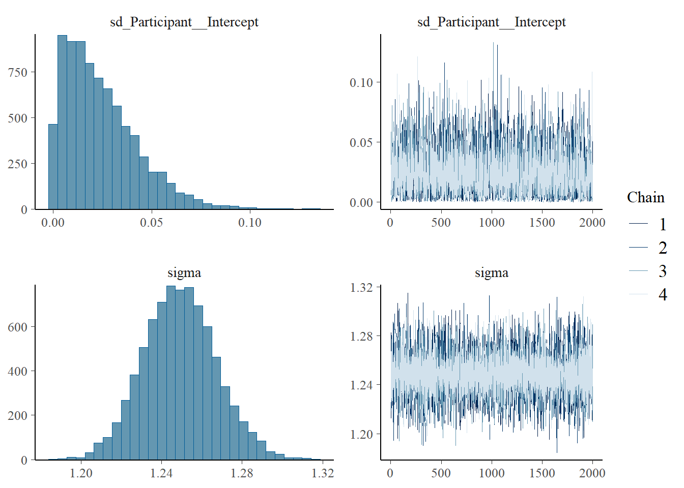
plot(h1.m1)
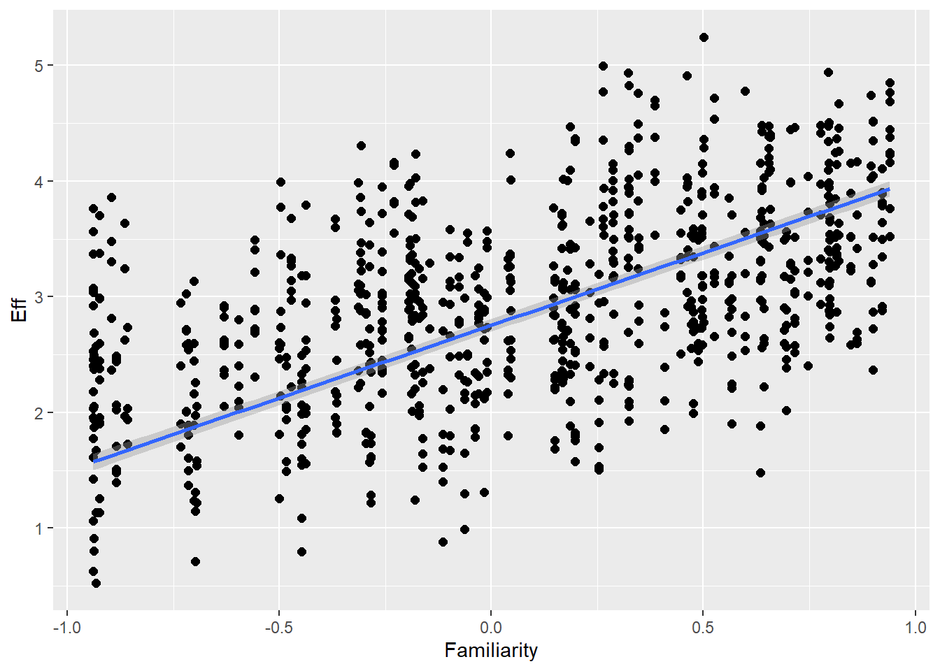
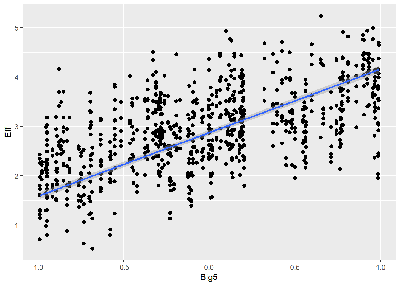
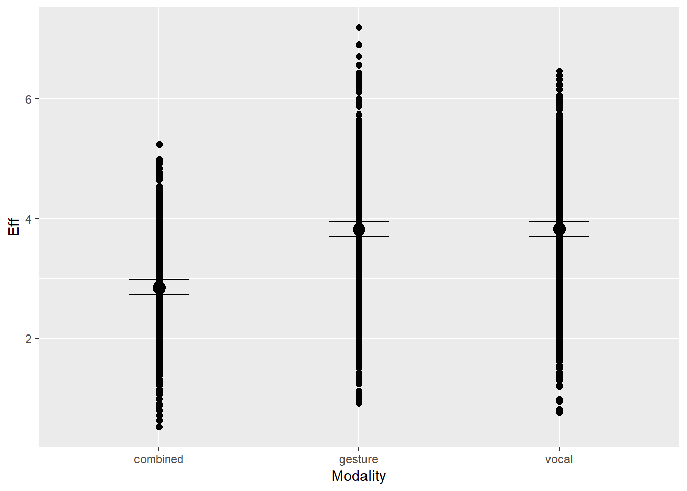
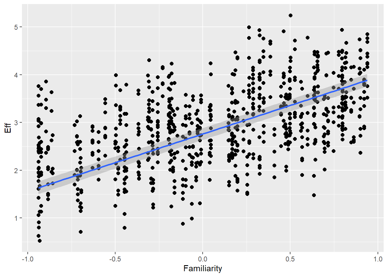
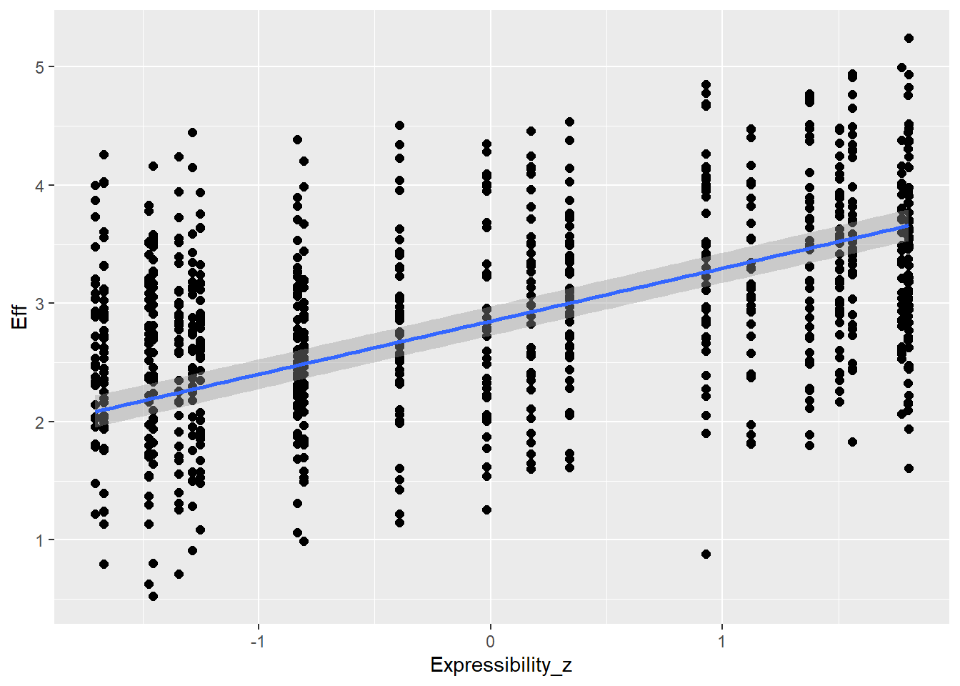
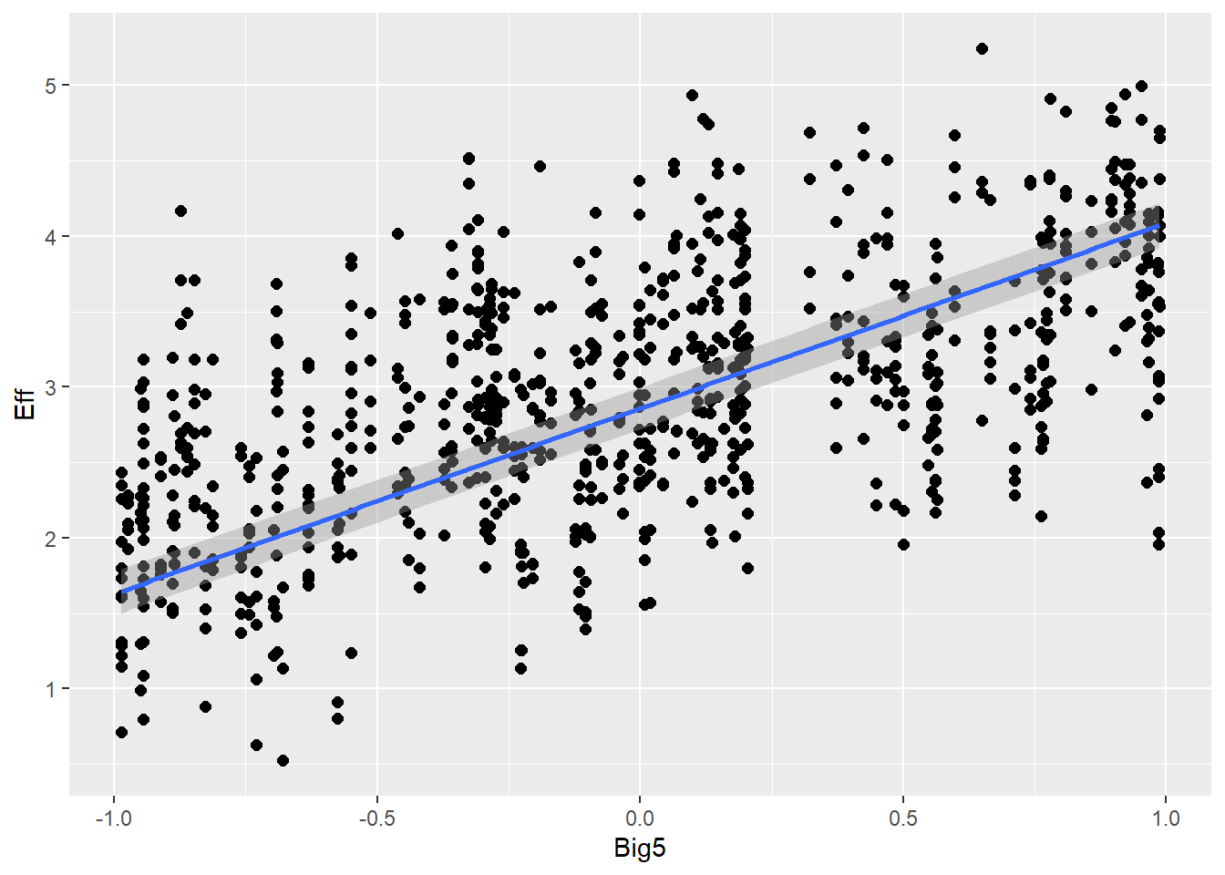
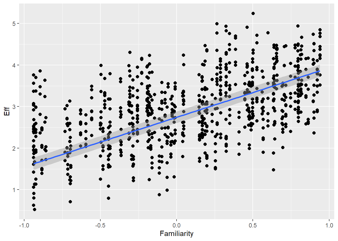
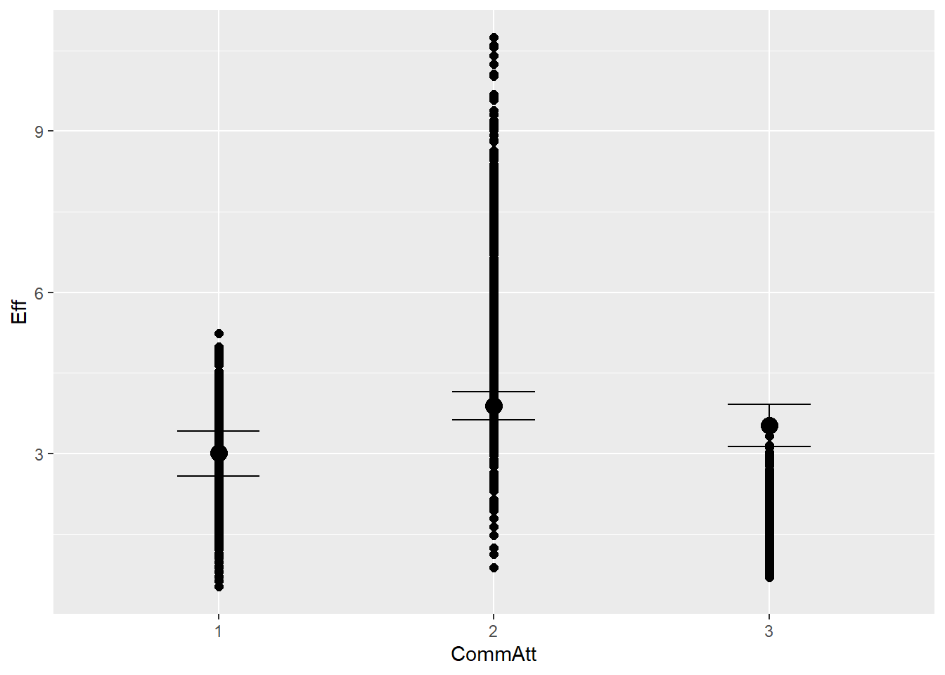
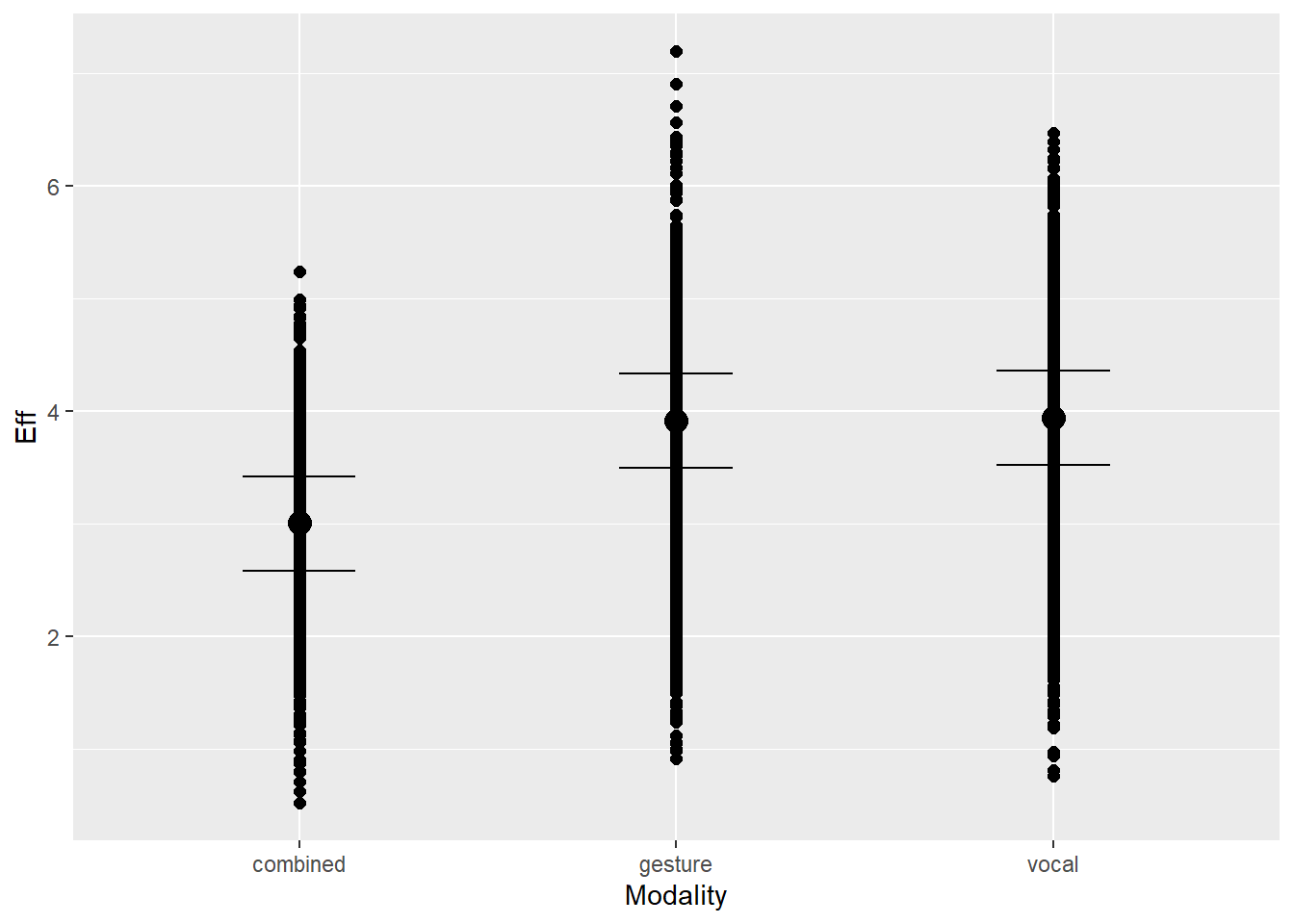
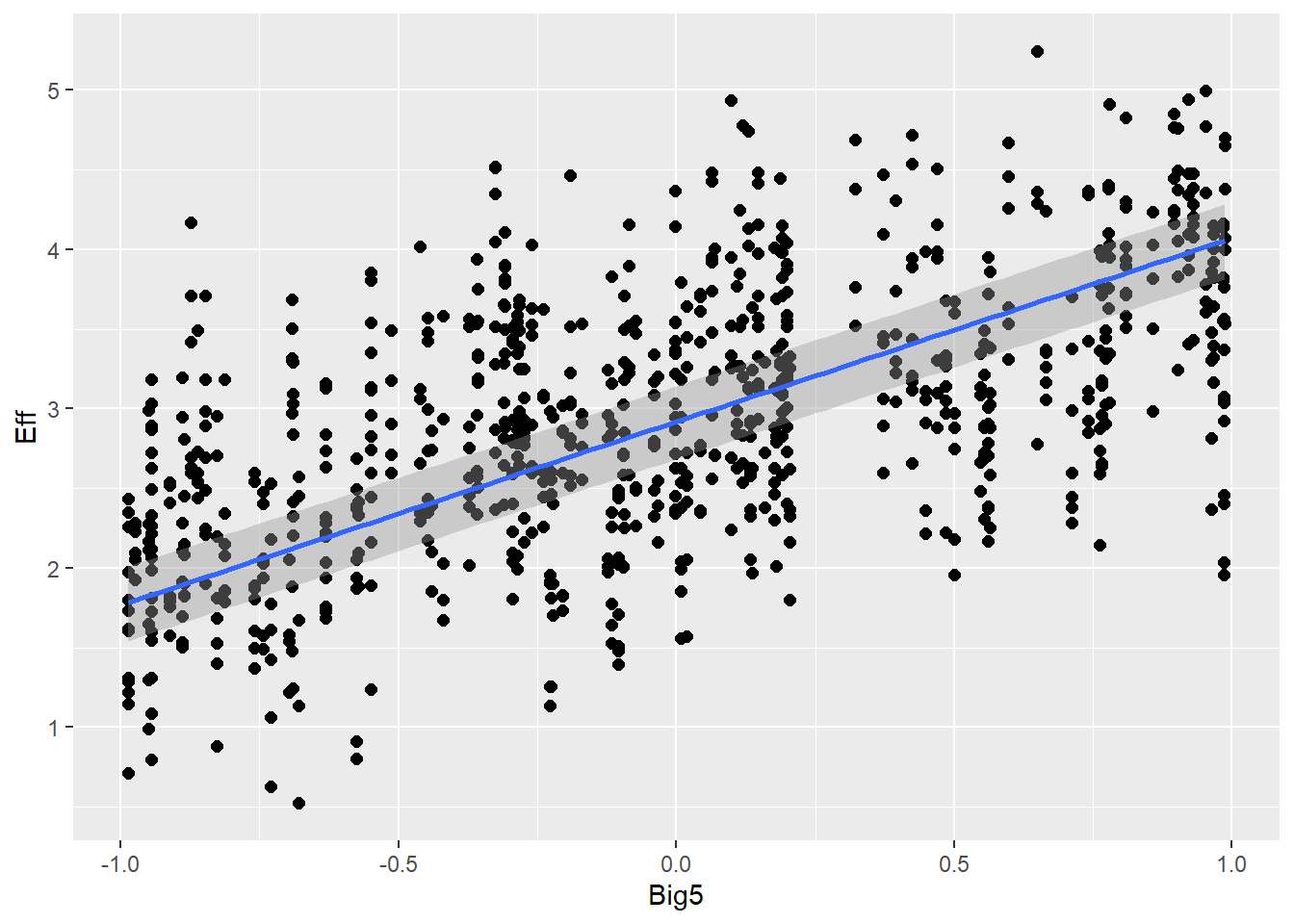
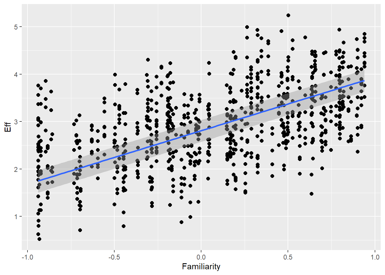
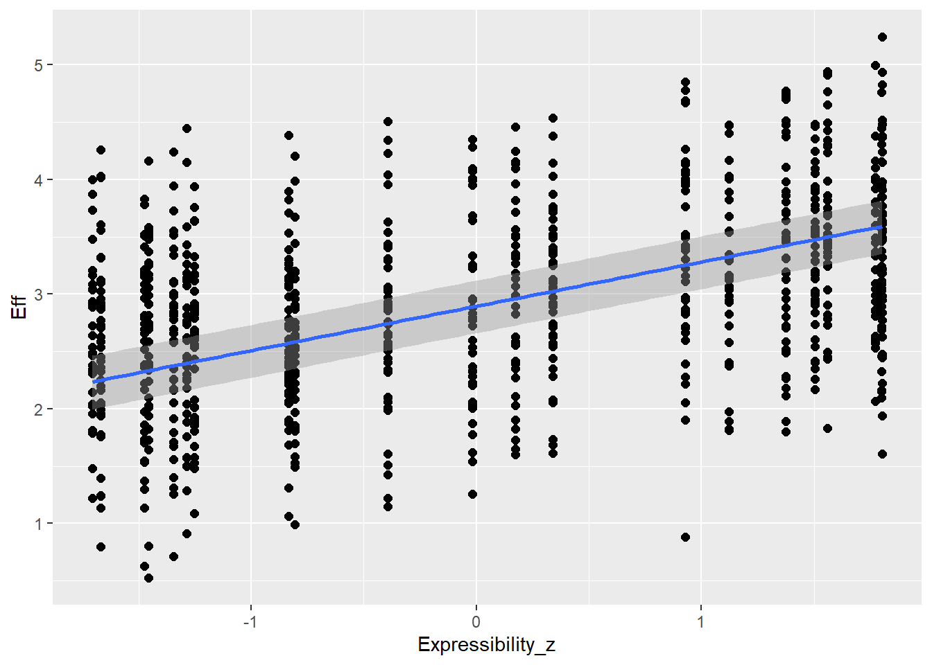
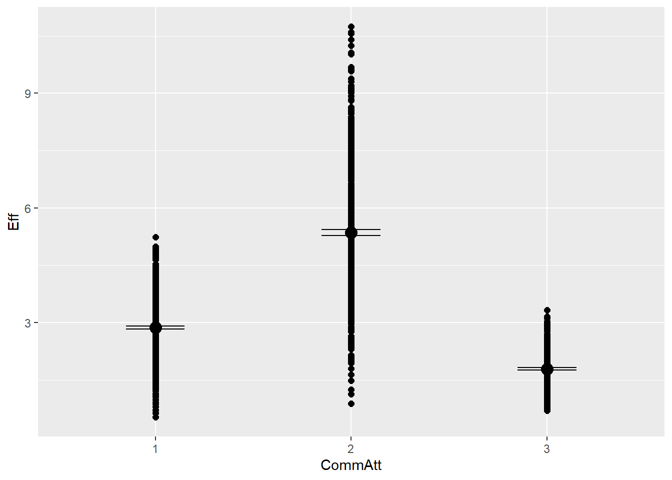
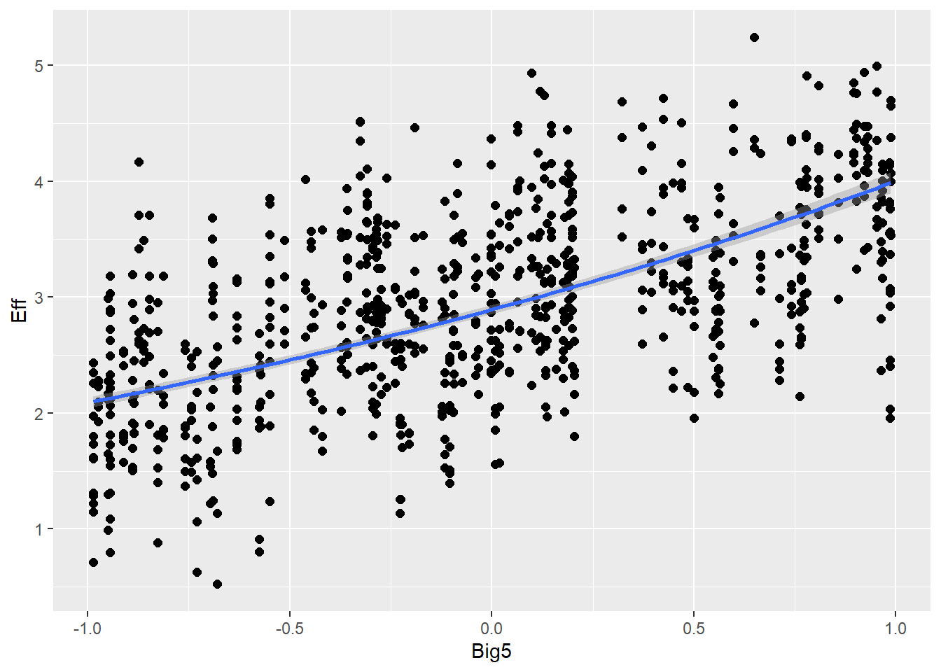
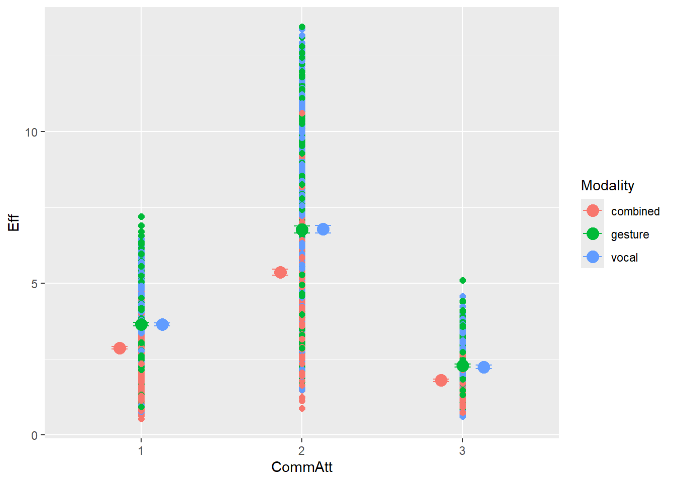
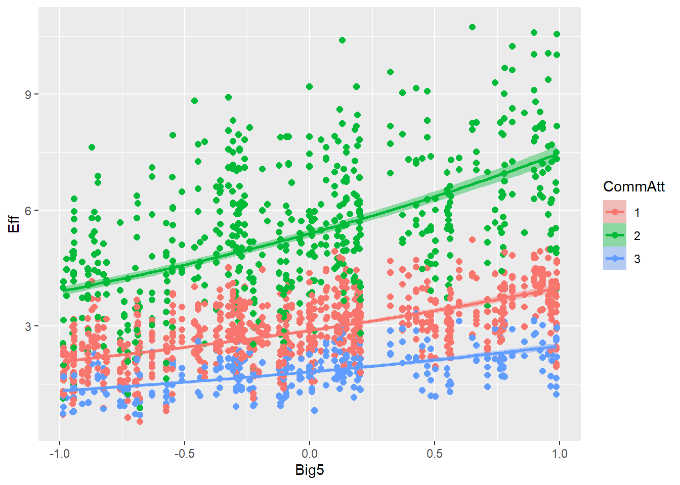
# all caterpillars look niceplot(conditional_effects(h1.m1), points =TRUE)
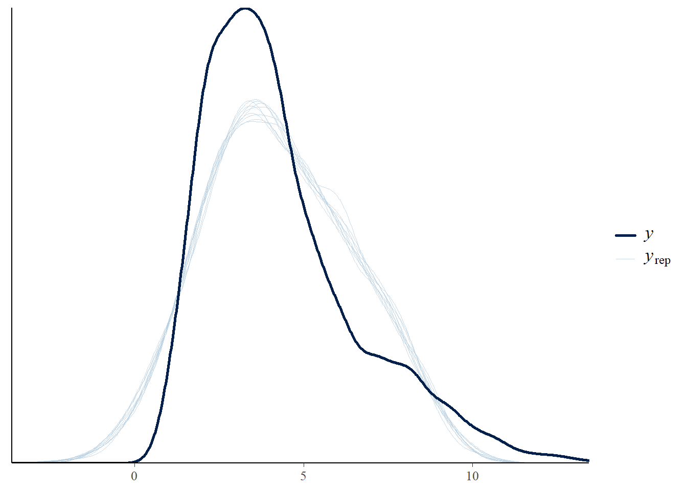
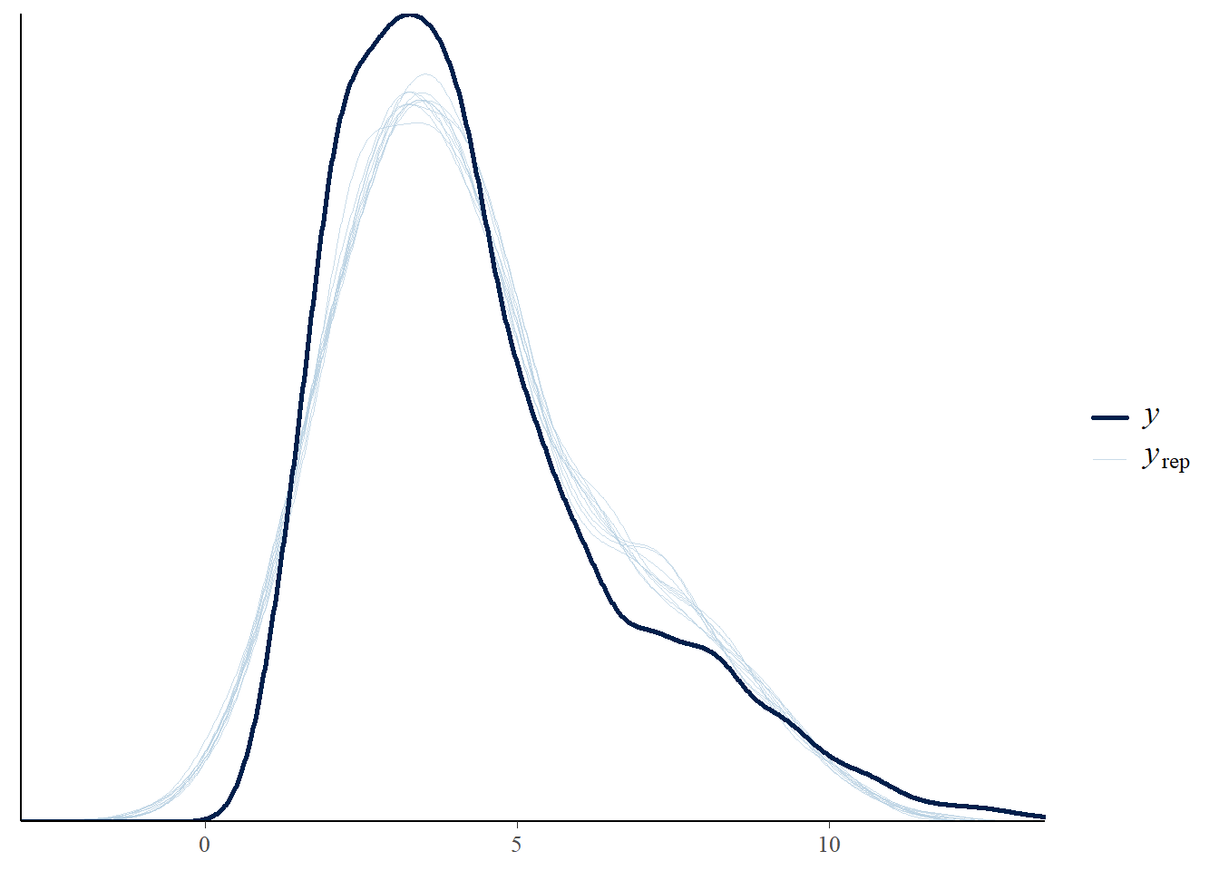
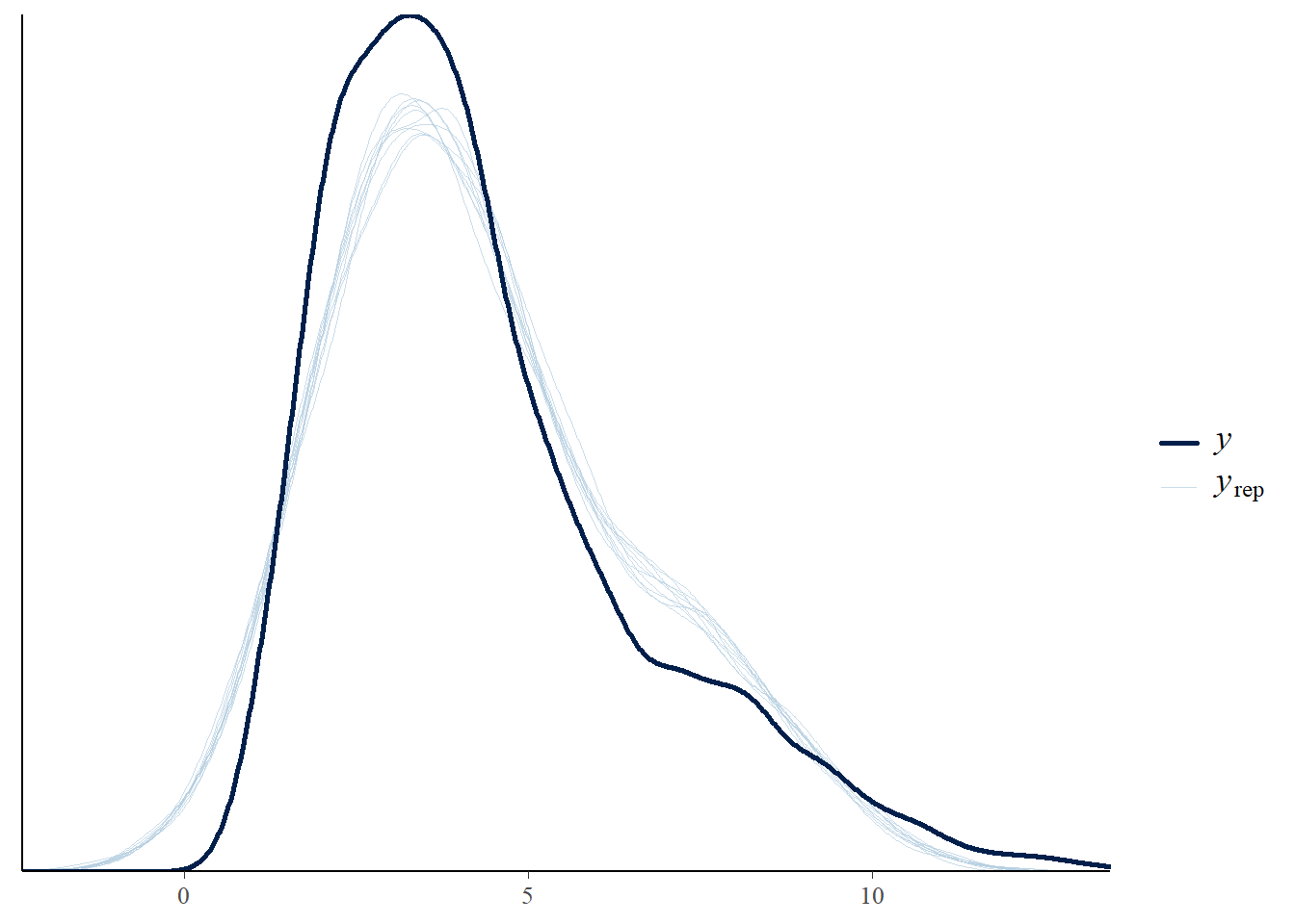
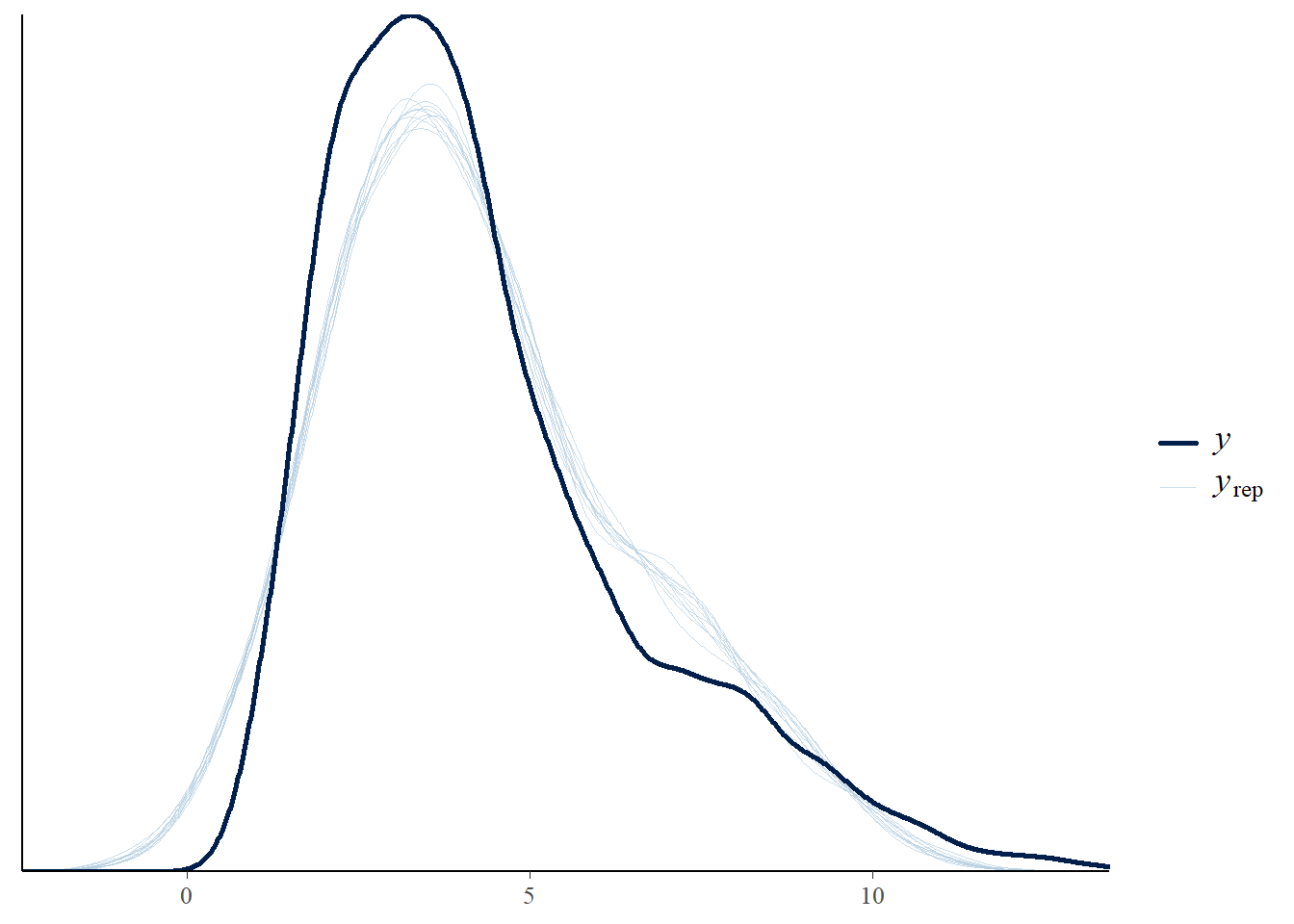
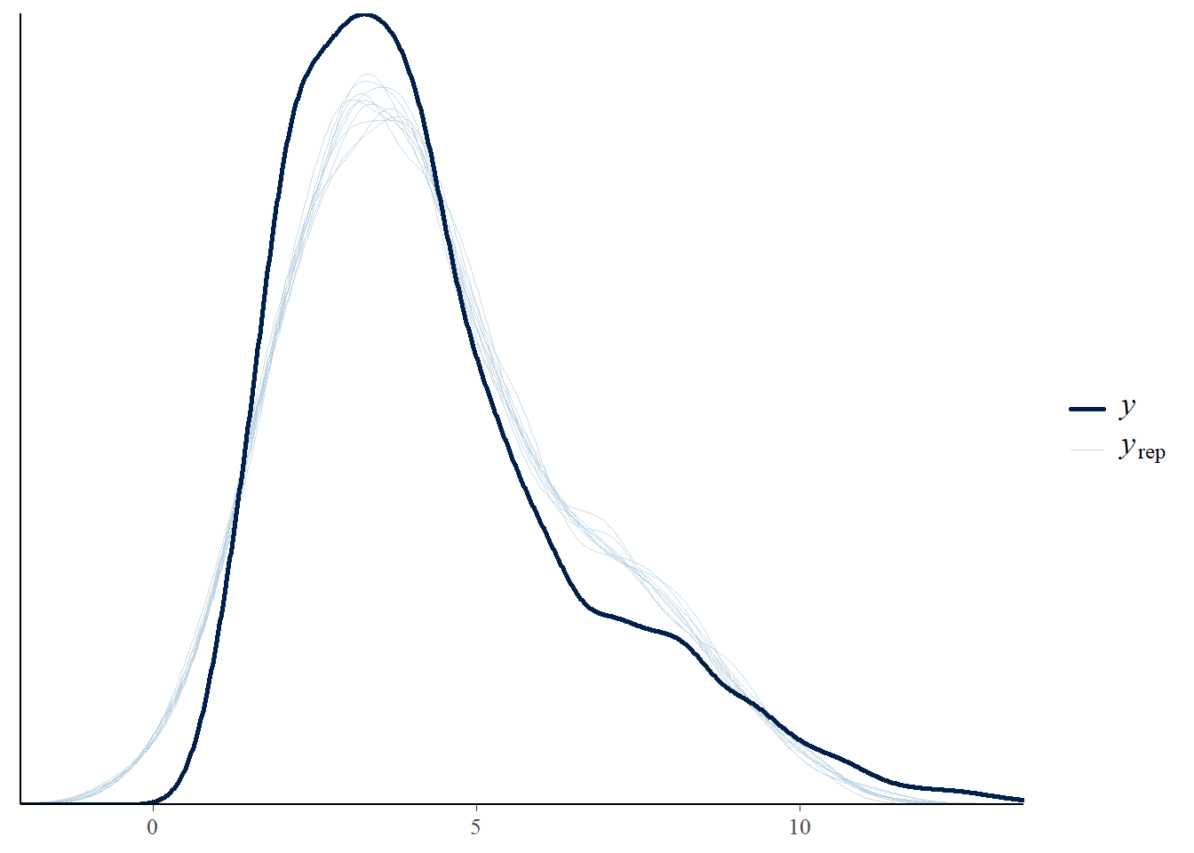
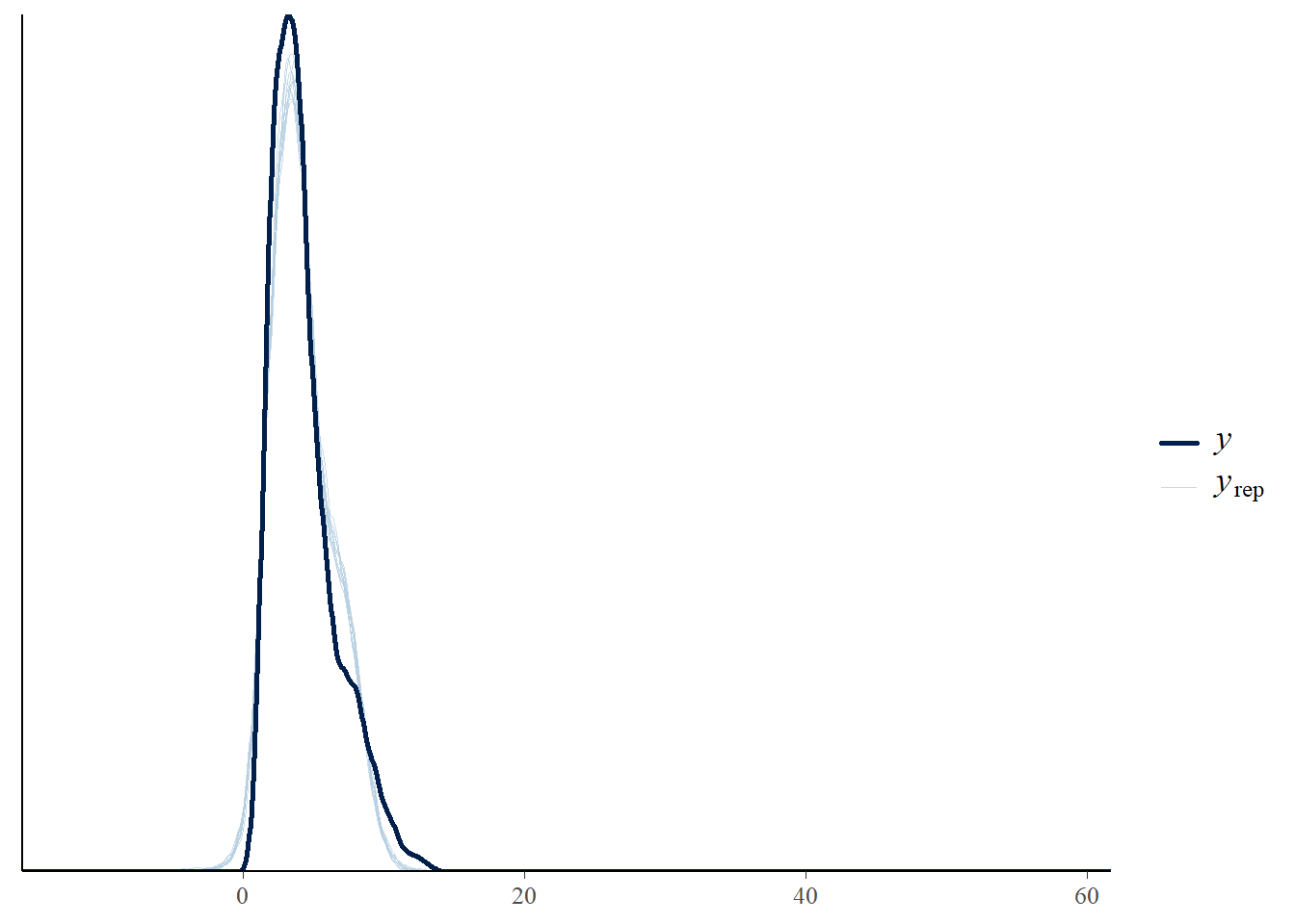
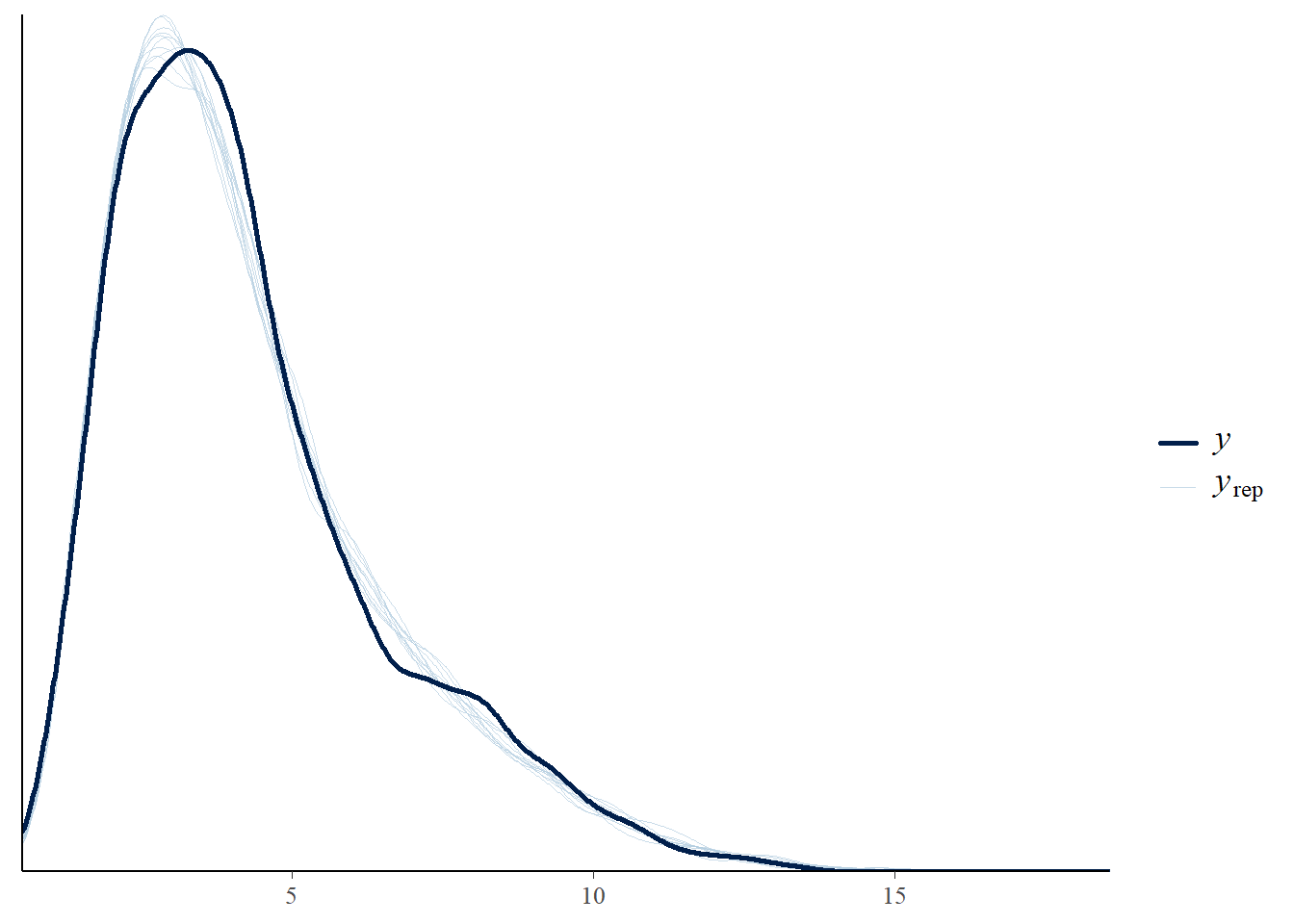
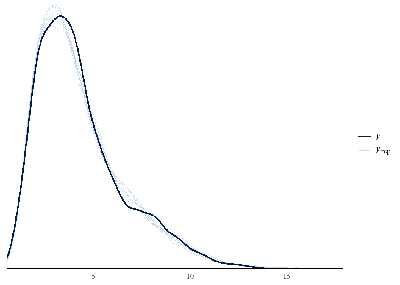
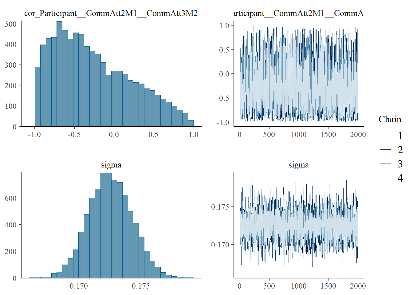
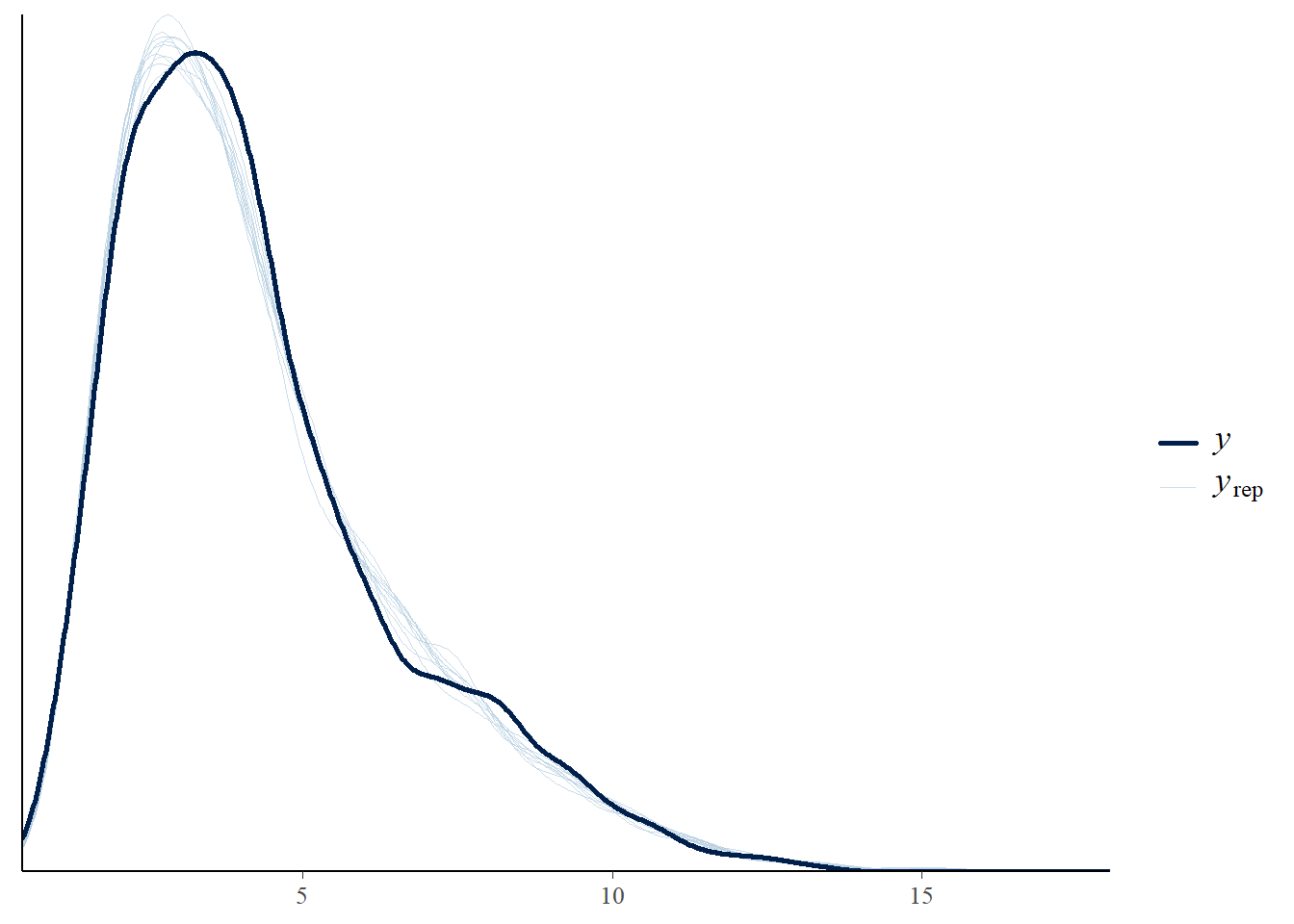
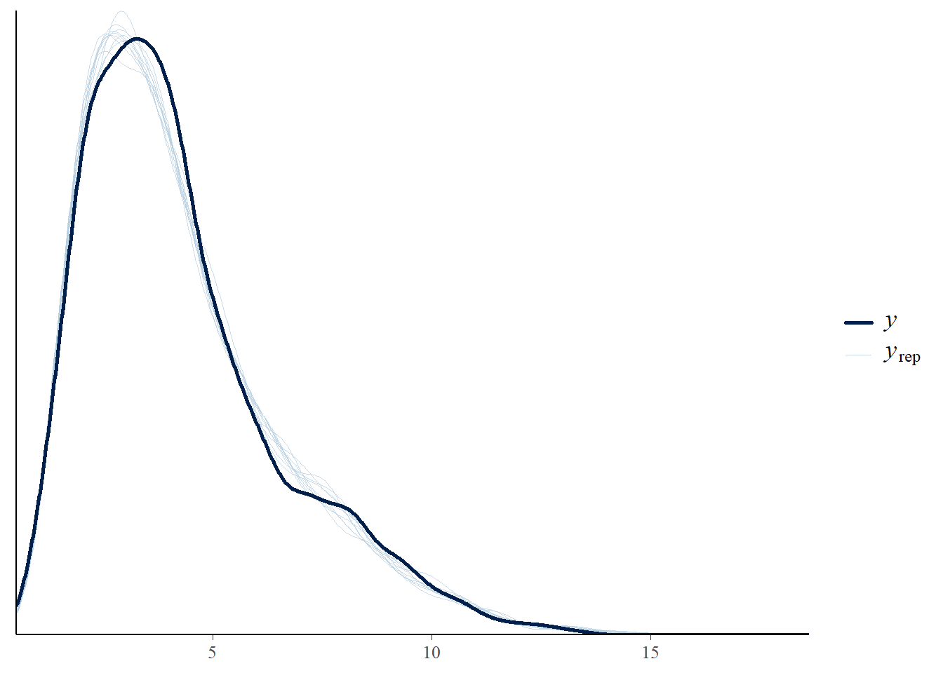
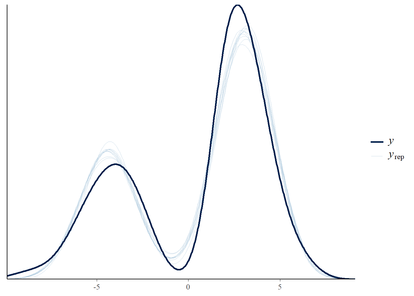
# the effects all go in good directionpp_check(h1.m1, type ="dens_overlay")
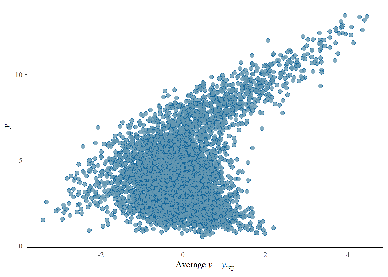
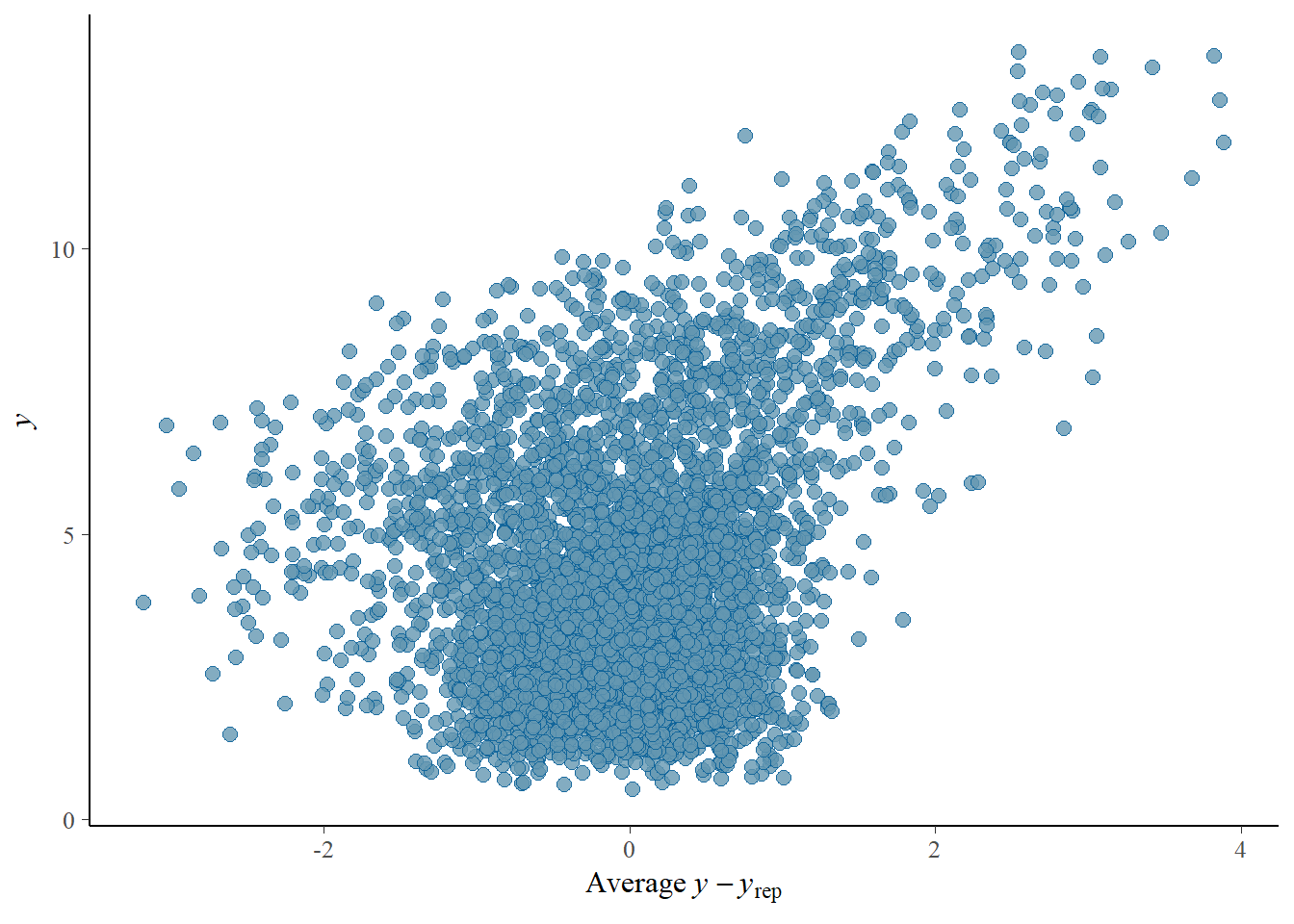
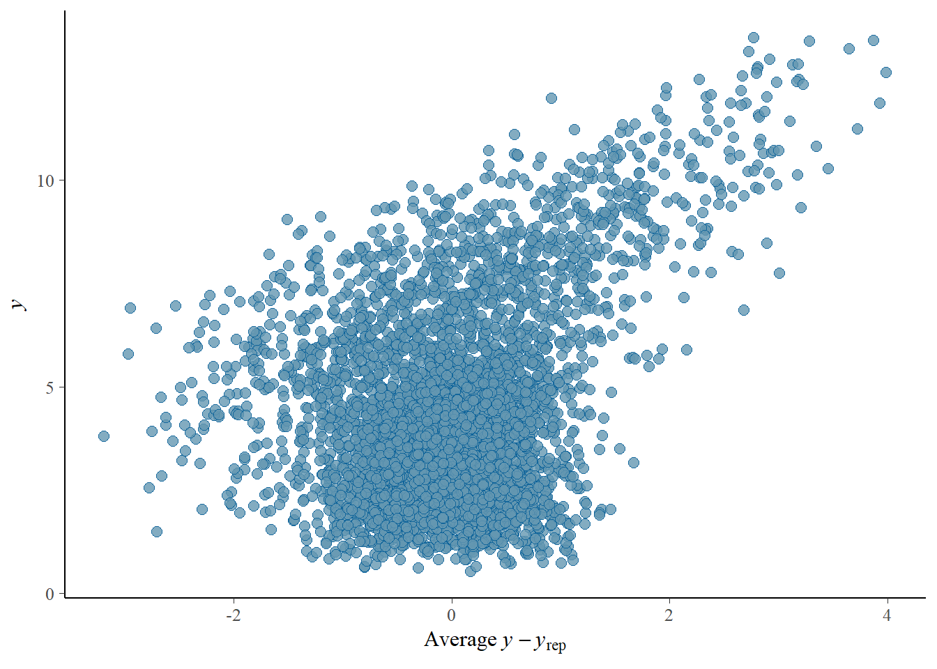
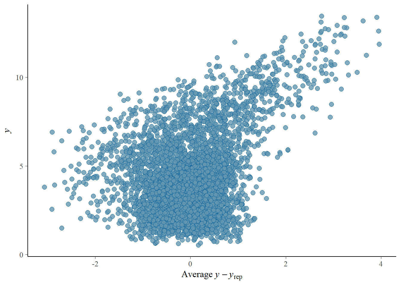
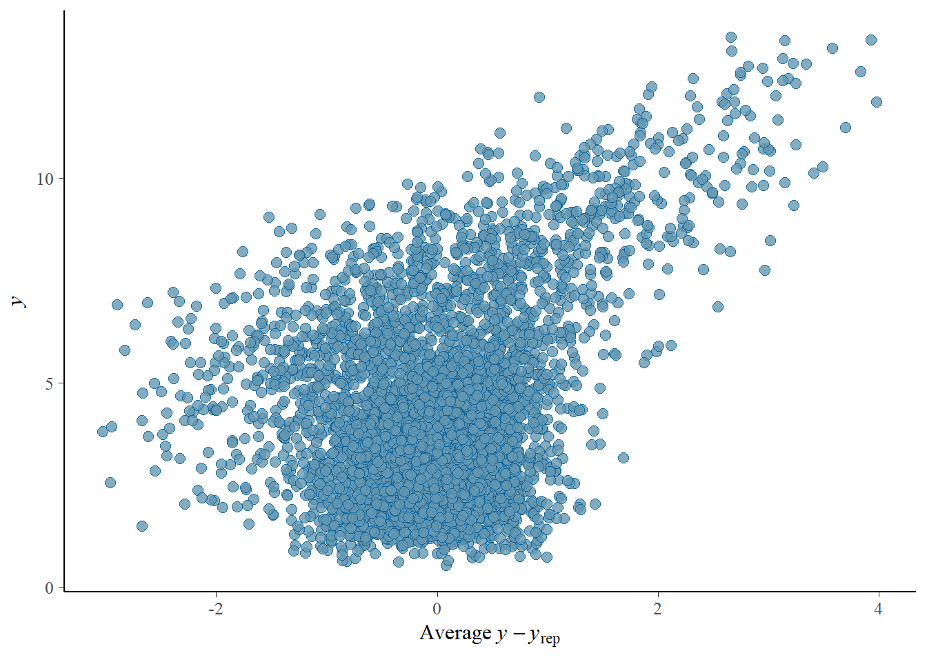
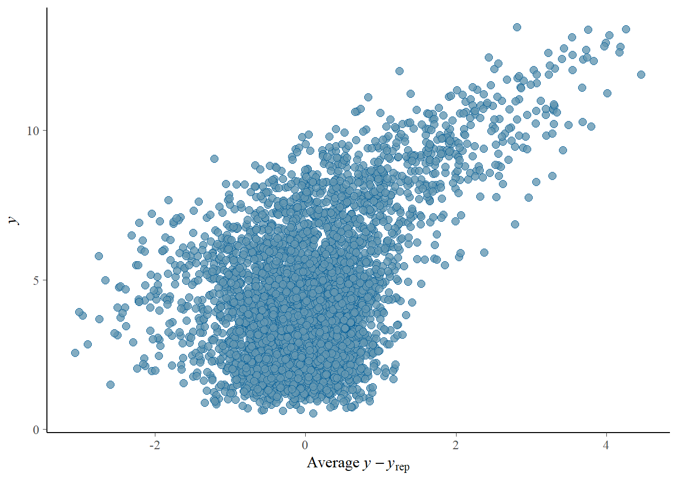
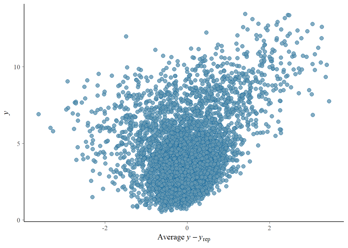
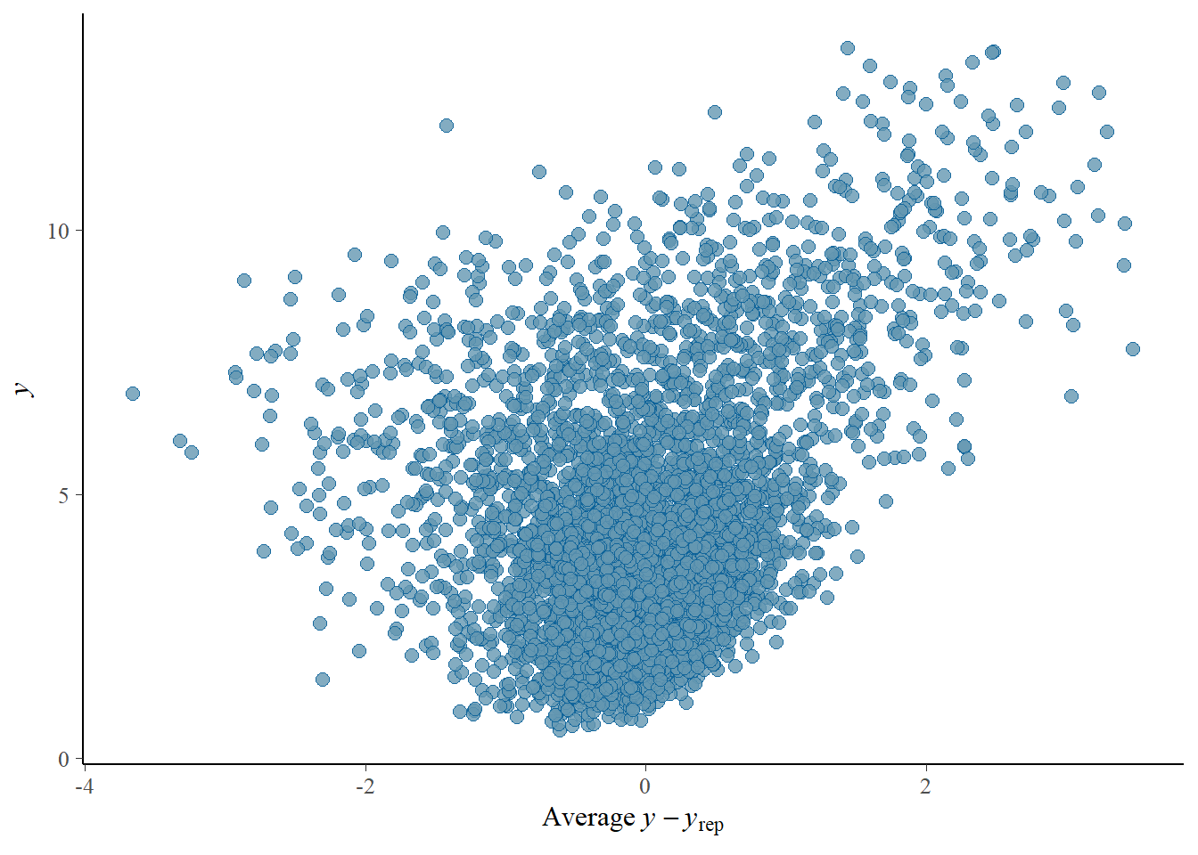
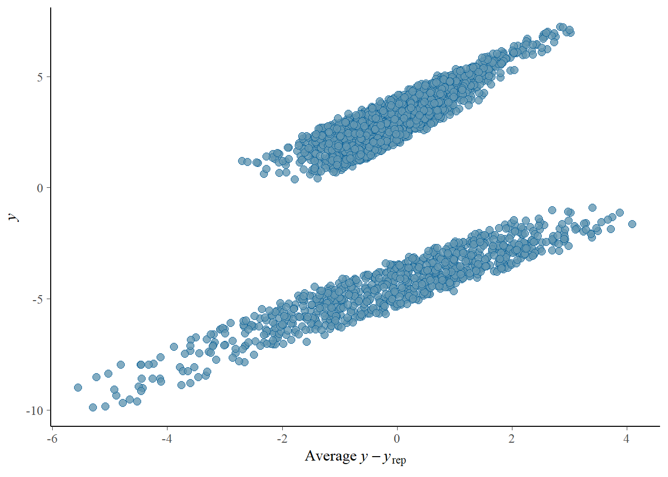
# Looks good but not amazing - mostly because the posteriors seem to not know effort cannot be negativepp_check(h1.m1, type ="error_scatter_avg")
# half blobby, half correlated, so still some room for improvement# positive correlation means that errors increase with predicted values. So the model does perform well for some range, but becomes less reliable with increase in the predicted values# also the blob is centered around 0 which is good# it could be we are ignoring some interaction terms or non-linearity (which we know we kind of do). Transformation could also help (e.g., log). Of course, we are also still not specifying any priors so let's not yet make it a disasterh1.m1_R2
Overall, we see good directions of all predictors, mostly also in accordance with the expected coefficients. Of course, the synthetic data is quite complex so there might be other dependencies that moderate the causal relationships and that is why we do not see exactly the numbers we use to create the data.
Let’s have another model for comparison.
We can assume that participants and concept have not only different baselines of effort (varying intercept). The effect of CommAtt on effort might vary across them too, hence we can try to add varying slopes for them and see whether the diagnostics improves. We will also add TrialNumber as a varying intercept, because we expect variation between earlier and later performances (because of learning, or opposite, fatigue).
Model 2 - Varying slopes and intercepts
h1.m2 <-brm(Eff ~1+ CommAtt + Modality + Big5 + Familiarity + Expressibility_z + (1+ CommAtt | Participant) + (1+ CommAtt | Concept) + (1| TrialNumber_c), data = final_data,iter =4000,cores =4)# Add criterions for later diagnosticsh1.m2 <-add_criterion(h1.m2, criterion =c("loo", "waic"))# Calculate also variance explained (R^2)h1.m2_R2 <-bayes_R2(h1.m2)# Save both as objectssaveRDS(h1.m2, here("09_Analysis_Modeling", "models", "h1.m2.rds"))saveRDS(h1.m2_R2, here("09_Analysis_Modeling", "models", "h1.m2_R2.rds"))beep(5)
One of the reasons why we might be getting the divergent transition is because of the correlation between slopes and intercepts in the previous model. Let’s now get rid of it
Model 3 - No correlation coefficient
h1.m3 <-brm(Eff ~1+ CommAtt + Modality + Big5 + Familiarity + Expressibility_z + (1+ CommAtt || Participant) + (1+ CommAtt || Concept) + (1|| TrialNumber_c), data = final_data,iter =4000,cores =4)# Add criterions for later diagnosticsh1.m3 <-add_criterion(h1.m3, criterion =c("loo", "waic"))# Calculate also variance explained (R^2)h1.m3_R2 <-bayes_R2(h1.m3)# Save both as objectssaveRDS(h1.m3, here("09_Analysis_Modeling", "models", "h1.m3.rds"))saveRDS(h1.m3_R2, here("09_Analysis_Modeling", "models", "h1.m3_R2.rds"))beep(5)
Now we will add some minimal priors, giving the model some reasonably informative, yet weak information.
priors_h1m3p <-c(set_prior("normal(2.5, 0.5)", class ="Intercept", lb=0),set_prior("normal(0,0.50)", class ="b", coef ="CommAtt2M1"),set_prior("normal(0,0.50)", class ="b", coef ="CommAtt3M2"),set_prior("normal(0,0.25)", class ="b", coef ="Modality1"),set_prior("normal(0,0.25)", class ="b", coef ="Modality2"),set_prior("normal(0,0.25)", class ="b", coef ="Big5"),set_prior("normal(0,0.25)", class ="b", coef ="Familiarity"),set_prior("normal(0,0.25)", class ="b", coef ="Expressibility_z"),set_prior("normal(0.5,0.1)", class ="sd", group ="TrialNumber_c"),set_prior("normal(0.5,0.1)", class ="sd", group ="Participant"),set_prior("normal(0.5,0.1)", class ="sd", group ="Concept"),set_prior("normal(1,0.1)", class ="sd"),set_prior("normal(0.5,0.25)", class ="sigma"))h1.m3p <-brm(Eff ~1+ CommAtt + Modality + Big5 + Familiarity + Expressibility_z + (1+ CommAtt || Participant) + (1+ CommAtt || Concept) + (1|| TrialNumber_c), data = final_data,prior=priors_h1m3p,family = gaussian,iter =4000,cores =4)# Add criterions for later diagnosticsh1.m3p <-add_criterion(h1.m3p, criterion =c("loo", "waic"))# Calculate also variance explained (R^2)h1.m3p_R2 <-bayes_R2(h1.m3p)# Save both as objectssaveRDS(h1.m3p, here("09_Analysis_Modeling", "models", "h1.m3p.rds"))saveRDS(h1.m3p_R2, here("09_Analysis_Modeling", "models", "h1.m3p_R2.rds"))beep(5)
Model 4 - Restricting priors with exponential distribution
Let’s do one more test with the priors, restricting sd them with exponential distribution, i.e., negative values are not possible
priors_h1m4 <-c(set_prior("normal(3, 0.3)", class ="Intercept", lb =0),set_prior("normal(0, 0.25)", class ="b", coef ="CommAtt2M1"),set_prior("normal(0, 0.25)", class ="b", coef ="CommAtt3M2"),set_prior("normal(0, 0.15)", class ="b", coef ="Modality1"),set_prior("normal(0, 0.15)", class ="b", coef ="Modality2"),set_prior("normal(0, 0.15)", class ="b", coef ="Big5"),set_prior("normal(0, 0.15)", class ="b", coef ="Familiarity"),set_prior("normal(0, 0.15)", class ="b", coef ="Expressibility_z"),# Exponential priors for standard deviationsset_prior("exponential(3)", class ="sd", group ="TrialNumber_c"), # exp(3) has a mean of 1/3 and concentrates most density around small valuesset_prior("exponential(3)", class ="sd", group ="Participant"),set_prior("exponential(3)", class ="sd", group ="Concept"),set_prior("exponential(1)", class ="sd"), # Generic sd prior# Residual standard deviation - keep it narrowset_prior("normal(0.5, 0.1)", class ="sigma"))h1.m4 <-brm(Eff ~1+ CommAtt + Modality + Big5 + Familiarity + Expressibility_z + (1+ CommAtt || Participant) + (1+ CommAtt || Concept) + (1|| TrialNumber_c), data = final_data,prior=priors_h1m4,family = gaussian,iter =4000,cores =4)# Add criterions for later diagnosticsh1.m4 <-add_criterion(h1.m4, criterion =c("loo", "waic"))# Calculate also variance explained (R^2)h1.m4_R2 <-bayes_R2(h1.m4)# Save both as objectssaveRDS(h1.m4, here("09_Analysis_Modeling", "models", "h1.m4.rds"))saveRDS(h1.m4_R2, here("09_Analysis_Modeling", "models", "h1.m4_R2.rds"))beep(5)
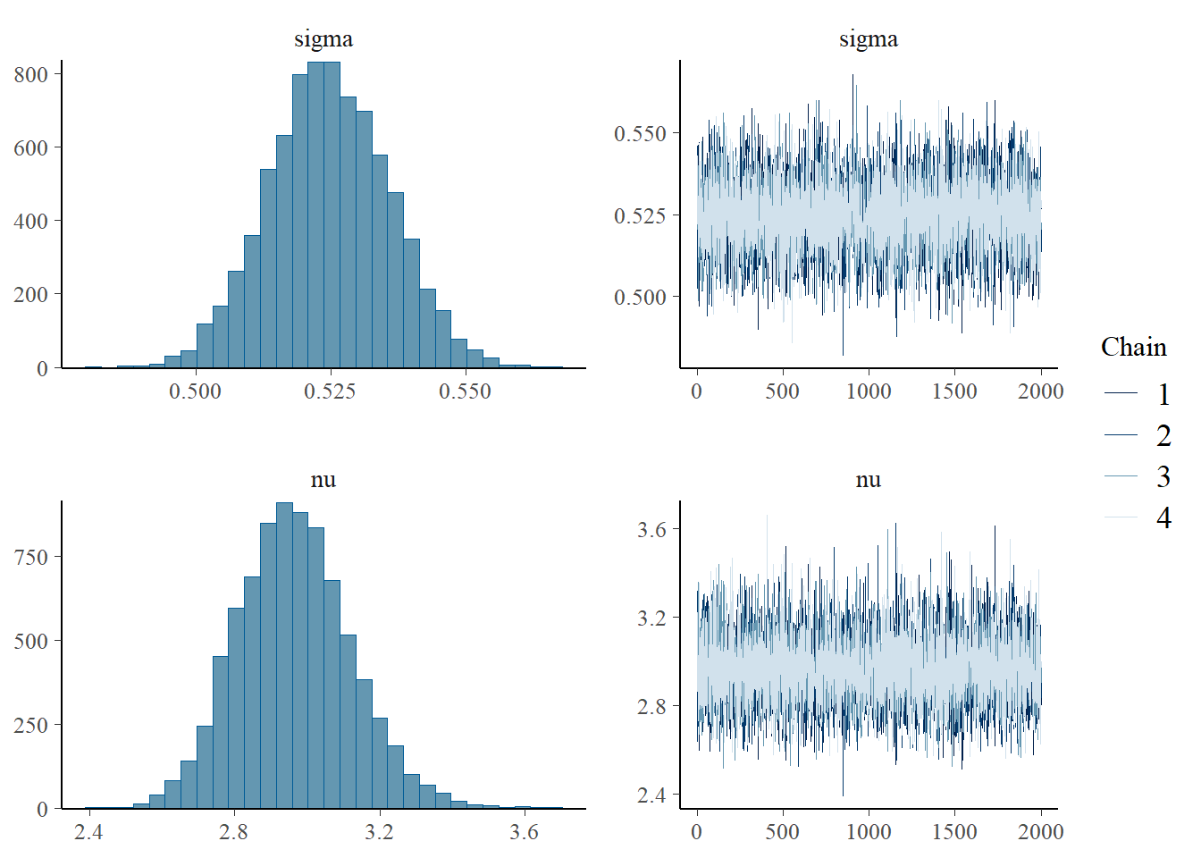
We still see negative values in the posterior simulations, so let’s try Student’s t-distribution which is more robust to outliers and can potentially reduce the likelihood of negative values (if we reduce degrees of freedom)
priors_h1m5 <-c(set_prior("normal(2.5, 0.5)", class ="Intercept", lb=0),set_prior("normal(0,0.50)", class ="b", coef ="CommAtt2M1"),set_prior("normal(0,0.50)", class ="b", coef ="CommAtt3M2"),set_prior("normal(0,0.25)", class ="b", coef ="Modality1"),set_prior("normal(0,0.25)", class ="b", coef ="Modality2"),set_prior("normal(0,0.25)", class ="b", coef ="Big5"),set_prior("normal(0,0.25)", class ="b", coef ="Familiarity"),set_prior("normal(0,0.25)", class ="b", coef ="Expressibility_z"),set_prior("normal(0.5,0.05)", class ="sd", group ="TrialNumber_c"),set_prior("normal(0.5,0.05)", class ="sd", group ="Participant"),set_prior("normal(0.5,0.05)", class ="sd", group ="Concept"),set_prior("normal(1,0.05)", class ="sd"),set_prior("normal(0.5,0.1)", class ="sigma"),set_prior("gamma(2, 0.1)", class ="nu") # Prior for degrees of freedom)h1.m5 <-brm(Eff ~1+ CommAtt + Modality + Big5 + Familiarity + Expressibility_z + (1+ CommAtt || Participant) + (1+ CommAtt || Concept) + (1|| TrialNumber_c), data = final_data,prior=priors_h1m5,family = student,iter =4000,cores =4)# Add criterions for later diagnosticsh1.m5 <-add_criterion(h1.m5, criterion =c("loo", "waic"))# Calculate also variance explained (R^2)h1.m5_R2 <-bayes_R2(h1.m5)# Save both as objectssaveRDS(h1.m5, here("09_Analysis_Modeling", "models", "h1.m5.rds"))saveRDS(h1.m5_R2, here("09_Analysis_Modeling", "models", "h1.m5_R2.rds"))beep(5)
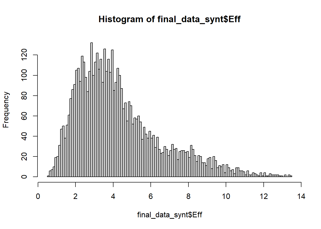
We have already seen - when plotting - that effort probably tends towards lognormal distribution. We will keep the model constant, just exchange the distribution. Priors are kept default
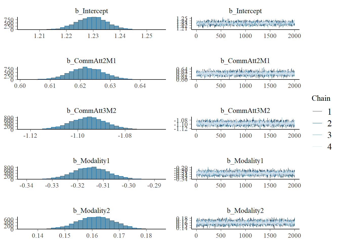
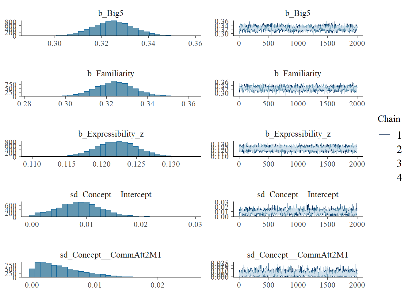
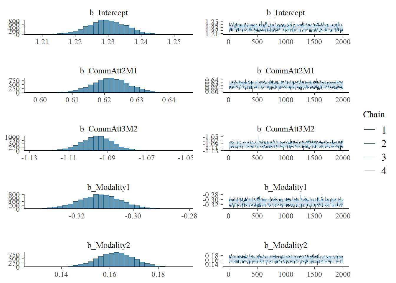
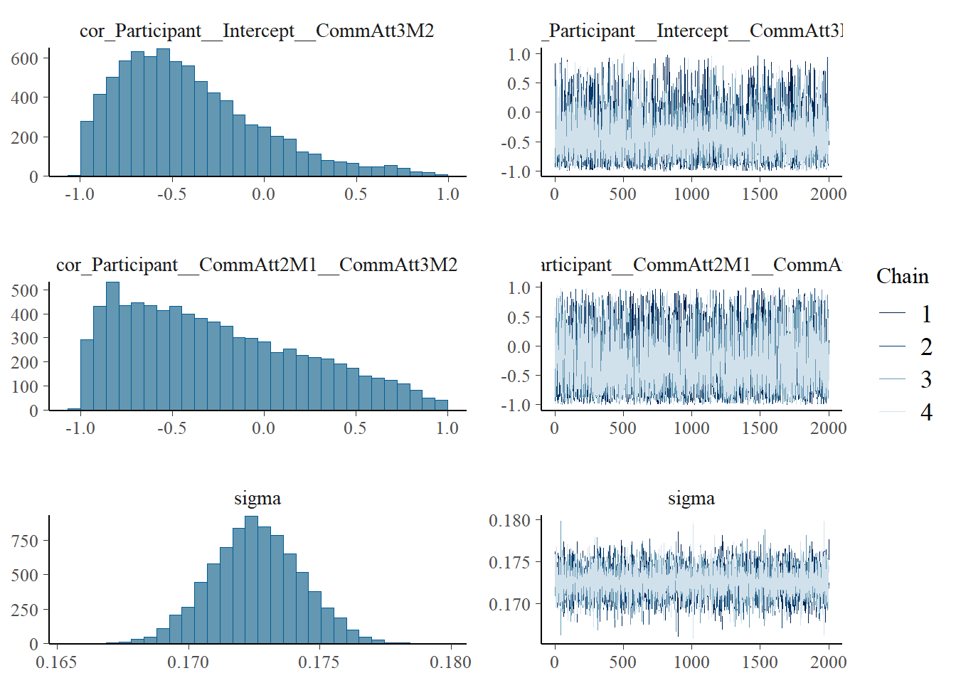
h1.m6 <-brm(Eff ~1+ CommAtt + Modality + Big5 + Familiarity + Expressibility_z + (1+ CommAtt || Participant) + (1+ CommAtt || Concept) + (1|| TrialNumber_c), data = final_data,family =lognormal(),iter =4000,cores =4)# Add criterions for later diagnosticsh1.m6 <-add_criterion(h1.m6, criterion =c("loo", "waic"))# Calculate also variance explained (R^2)h1.m6_R2 <-bayes_R2(h1.m6)# Save both as objectssaveRDS(h1.m6, here("09_Analysis_Modeling", "models", "h1.m6.rds"))saveRDS(h1.m6_R2, here("09_Analysis_Modeling", "models", "h1.m6_R2.rds"))beep(5)
 Family: lognormal
  Links: mu = identity; sigma = identity
Formula: Eff ~ 1 + CommAtt + Modality + Big5 + Familiarity + Expressibility_z + (1 + CommAtt || Participant) + (1 + CommAtt || Concept) + (1 || TrialNumber_c)
   Data: final_data (Number of observations: 5076)
  Draws: 4 chains, each with iter = 4000; warmup = 2000; thin = 1;
         total post-warmup draws = 8000

Multilevel Hyperparameters:
~Concept (Number of levels: 21)
               Estimate Est.Error l-95% CI u-95% CI Rhat Bulk_ESS Tail_ESS
sd(Intercept)      0.01      0.00     0.00     0.02 1.00     2298     2414
sd(CommAtt2M1)     0.00      0.00     0.00     0.01 1.00     4803     3682
sd(CommAtt3M2)     0.01      0.01     0.00     0.02 1.00     3687     3650

~Participant (Number of levels: 120)
               Estimate Est.Error l-95% CI u-95% CI Rhat Bulk_ESS Tail_ESS
sd(Intercept)      0.05      0.00     0.04     0.06 1.00     2844     4508
sd(CommAtt2M1)     0.00      0.00     0.00     0.01 1.00     4417     3655
sd(CommAtt3M2)     0.01      0.01     0.00     0.03 1.00     2618     2888

~TrialNumber_c (Number of levels: 50)
              Estimate Est.Error l-95% CI u-95% CI Rhat Bulk_ESS Tail_ESS
sd(Intercept)     0.00      0.00     0.00     0.01 1.00     3411     3578

Regression Coefficients:
                 Estimate Est.Error l-95% CI u-95% CI Rhat Bulk_ESS Tail_ESS
Intercept            1.23      0.01     1.22     1.24 1.00     3120     4439
CommAtt2M1           0.62      0.01     0.61     0.63 1.00     9634     6358
CommAtt3M2          -1.10      0.01    -1.11    -1.08 1.00     9514     5588
Modality1           -0.31      0.01    -0.33    -0.30 1.00     9097     6088
Modality2            0.16      0.01     0.15     0.17 1.00     9223     6512
Big5                 0.32      0.01     0.31     0.34 1.00     2924     4558
Familiarity          0.32      0.01     0.31     0.34 1.00     2297     3545
Expressibility_z     0.12      0.00     0.12     0.13 1.00    10923     6710

Further Distributional Parameters:
      Estimate Est.Error l-95% CI u-95% CI Rhat Bulk_ESS Tail_ESS
sigma     0.17      0.00     0.17     0.18 1.00    11348     5998

Draws were sampled using sampling(NUTS). For each parameter, Bulk_ESS
and Tail_ESS are effective sample size measures, and Rhat is the potential
scale reduction factor on split chains (at convergence, Rhat = 1).
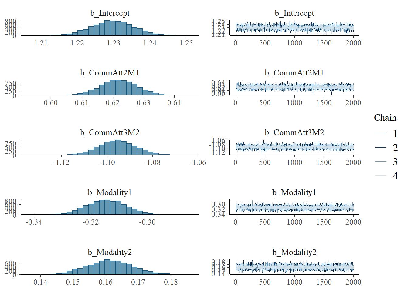
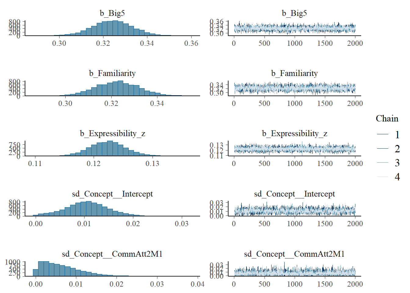
# Coefficients remain mostly unchanged
Converting to original scale
Of course now we have all on lognormal scale so it is not so straightforwadly interpretable. This is how we can get to the values of an effort under certain value of a predictor
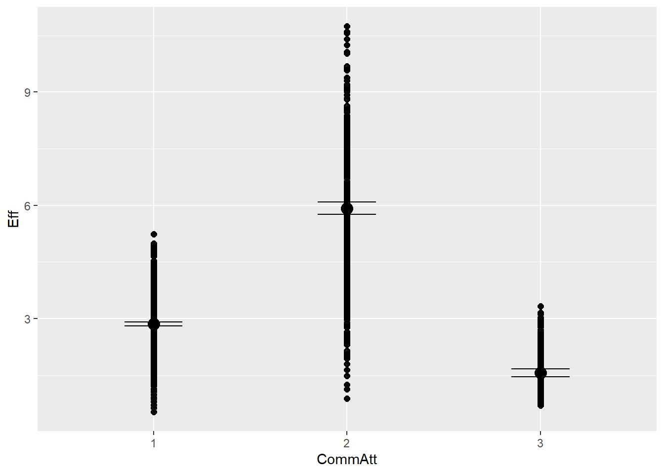
# Compute estimated marginal means on log-scaleem_h1.m6 <-emmeans(h1.m6, ~ CommAtt) #~ CommAtt#Backtransform the post.beta valuesem_h1.m6@post.beta <-exp(em_h1.m6@post.beta)print(em_h1.m6)
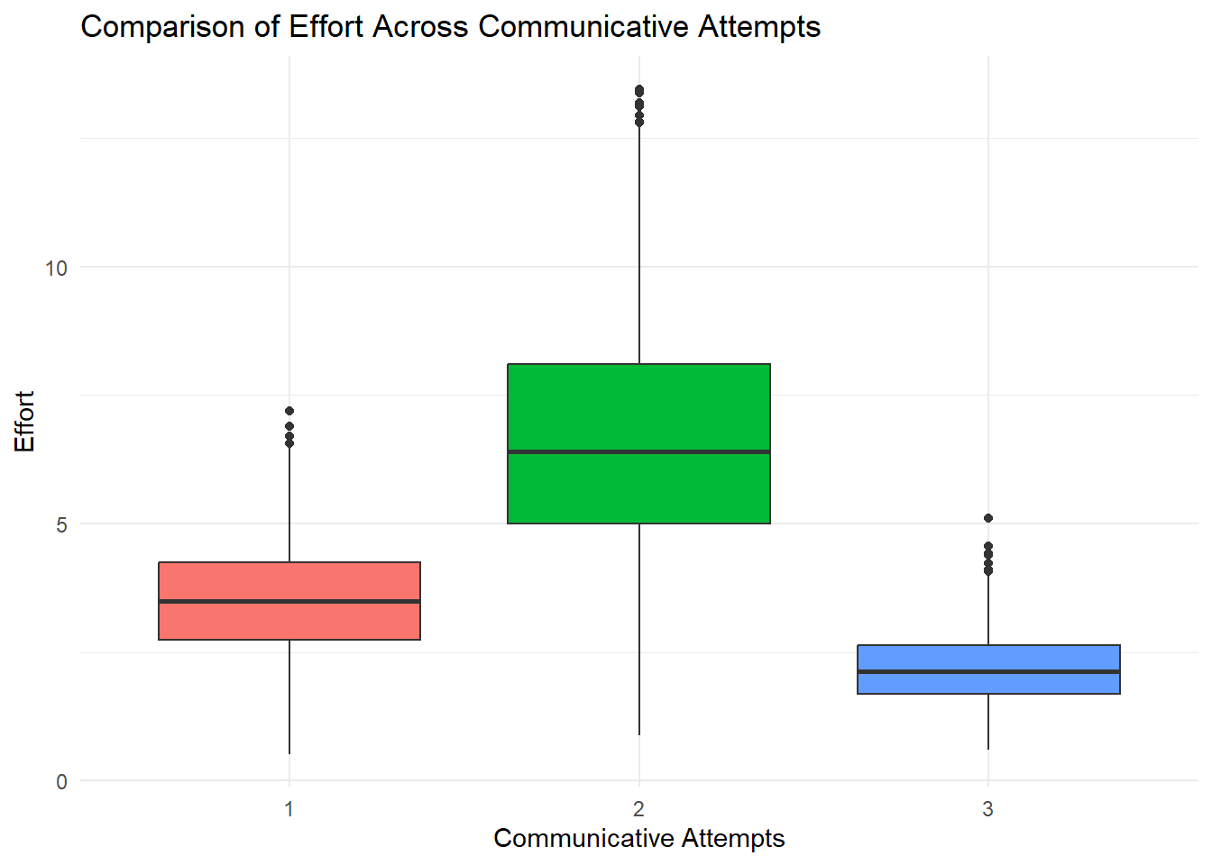
 CommAtt emmean lower.HPD upper.HPD
 1         3.33      3.29      3.37
 2         6.21      6.13      6.29
 3         2.08      2.05      2.11

Results are averaged over the levels of: Modality
Point estimate displayed: median
HPD interval probability: 0.95
So we indeed see that effort in CommAtt2 increase but then decreases again for CommAtt3. We can also try to get our simulated betas
coeff1 <-3.33*1.5coeff2 <-3.33*0.5print(coeff1)
[1] 4.995
print(coeff2) # which is very close to the mean values we see from the model
[1] 1.665
We see that the effect estimated by the model is now stronger than in our simulated data. However, note that these values are averaged over predictor modality
We can also try a different method to get the coefficients (code adapted from here)
# Extract posterior samplesalpha_samples <-as_draws_df(h1.m6)$b_Interceptbeta_2_vs_1 <-as_draws_df(h1.m6)$b_CommAtt2M1beta_3_vs_2 <-as_draws_df(h1.m6)$b_CommAtt3M2# Compute expected values on the log scalemu_1 <- alpha_samples # CommAtt 1mu_2 <- alpha_samples + beta_2_vs_1 # CommAtt 2mu_3 <- alpha_samples + beta_2_vs_1 + beta_3_vs_2 # CommAtt 3# Transform to original scaleeffect_1 <-exp(mu_1)effect_2 <-exp(mu_2)effect_3 <-exp(mu_3)# Calculate contrasts on the original scaleeffect_diff_2_vs_1 <- effect_2 - effect_1effect_diff_3_vs_2 <- effect_3 - effect_2effect_diff_3_vs_1 <- effect_3 - effect_1# Summarize the effectslist(mean_intercept =mean(effect_1),mean_diff_2_vs_1 =c(mean =mean(effect_diff_2_vs_1), quantile(effect_diff_2_vs_1, c(0.025, 0.975))),mean_diff_3_vs_2 =c(mean =mean(effect_diff_3_vs_2), quantile(effect_diff_3_vs_2, c(0.025, 0.975))),mean_diff_3_vs_1 =c(mean =mean(effect_diff_3_vs_1), quantile(effect_diff_3_vs_1, c(0.025, 0.975))))
$mean_intercept
[1] 3.419549

$mean_diff_2_vs_1
    mean     2.5%    97.5%
2.950688 2.872812 3.029410

$mean_diff_3_vs_2
     mean      2.5%     97.5%
-4.240333 -4.321665 -4.160104

$mean_diff_3_vs_1
     mean      2.5%     97.5%
-1.289646 -1.320918 -1.257698
Now we can use these coefficients to transform to our simulated betas
All models seems actually ok in terms of Rhat values except model 2 (h1.m2)
ESS
Effective sample size tells how many independent samples the model has effectively drawn from the PD. Low ESS suggests autocorrelation (i.e., sample explores one part of posterior), while high ESS means good mix
# Extract n_eff values for each modelneff_ratio_list <-lapply(model_list, function(model) { neff_values <-neff_ratio(model) # Here we calculate ratio (not the raw number of effective samples)data.frame(model =deparse(substitute(model)), min_neff =min(neff_values), max_neff =max(neff_values),mean_neff =mean(neff_values))})# Combine and inspectdo.call(rbind, neff_ratio_list)
So there are some considerable differences for different coefficients
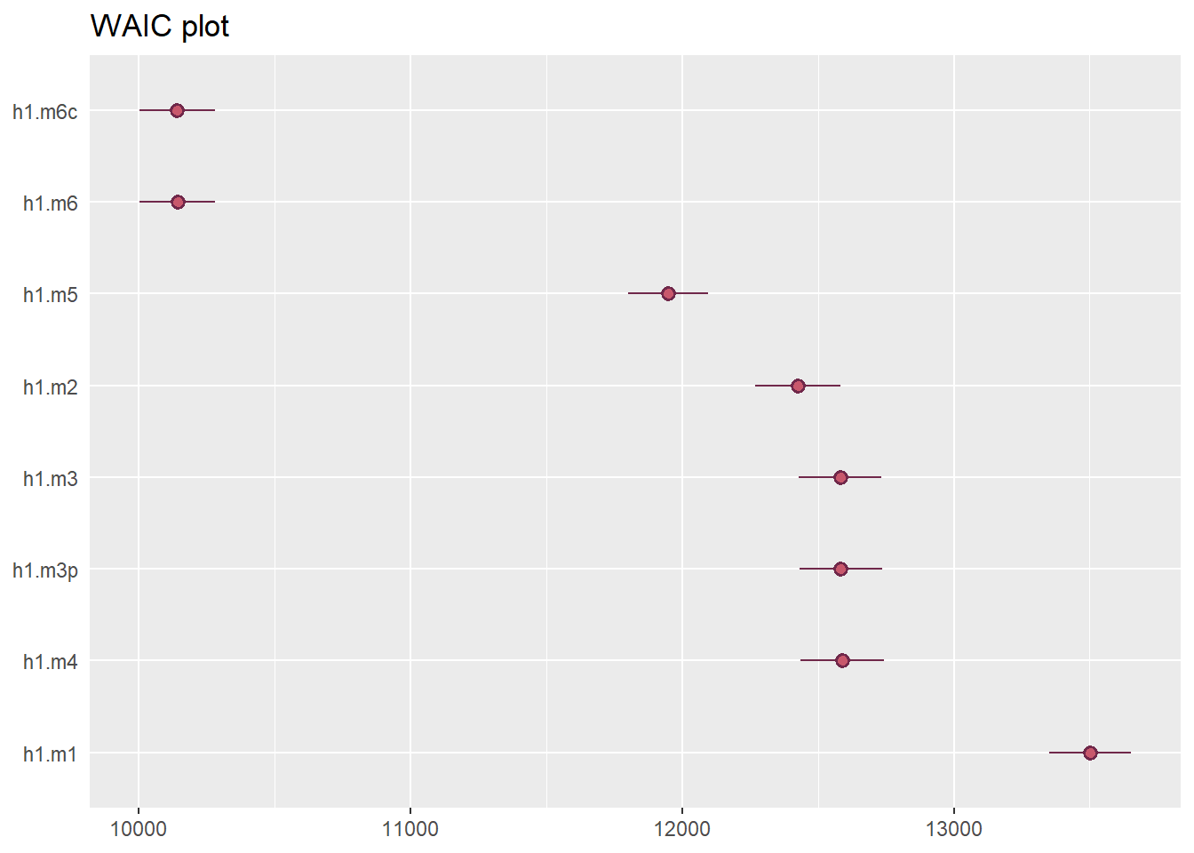
LOO & WAIC
Leave-One-Out (LOO) validation is a technique where, for each iteration, one data point is left out as the test set, and the model is trained on the remaining data points; this process is repeated for each data point, and the model’s overall performance is averaged over all iterations.
elpd_waic (expected log pointwise predictive density for WAIC): This represents the model’s predictive fit to the data. Higher values indicate a better fit.
se_elpd_waic (standard error of elpd_waic): Measures uncertainty around the elpd_waic estimate.
waic: The Widely Applicable Information Criterion, a measure of model fit where lower values indicate a better fit.
se_waic (standard error of WAIC): Uncertainty around the WAIC estimate.
elpd_diff: The difference in the elpd_waic between the model in question and the baseline model (fit_eff_2, which has elpd_diff of 0). A negative value indicates that the model fits worse than fit_eff_2.
se_diff: The standard error of the elpd_diff, indicating how much uncertainty there is in the difference in predictive performance.
p_waic: The number of effective parameters in the model (related to model complexity). Lower values indicate simpler models, and higher values suggest more complexity.
So as ppcheck already suggested, lognormal model indeed seem to have the most predictive power. For this particular (synthetic) data, we will now proceed with model h1.m6c
We will first add some mildly informative priors, and then we also try to add some interaction terms and do a comparison once again.
Model 7 - lognormal with priors
Let’s first check what priors have been selected as default for h1.m6c
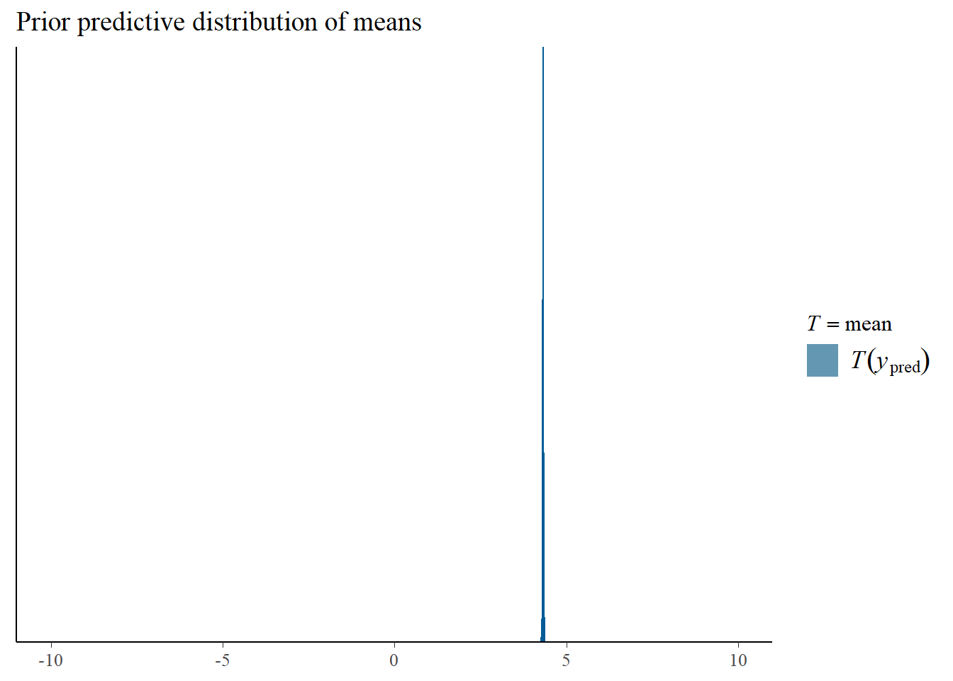
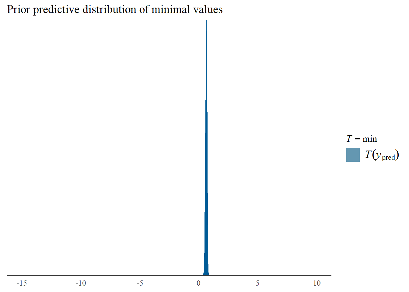
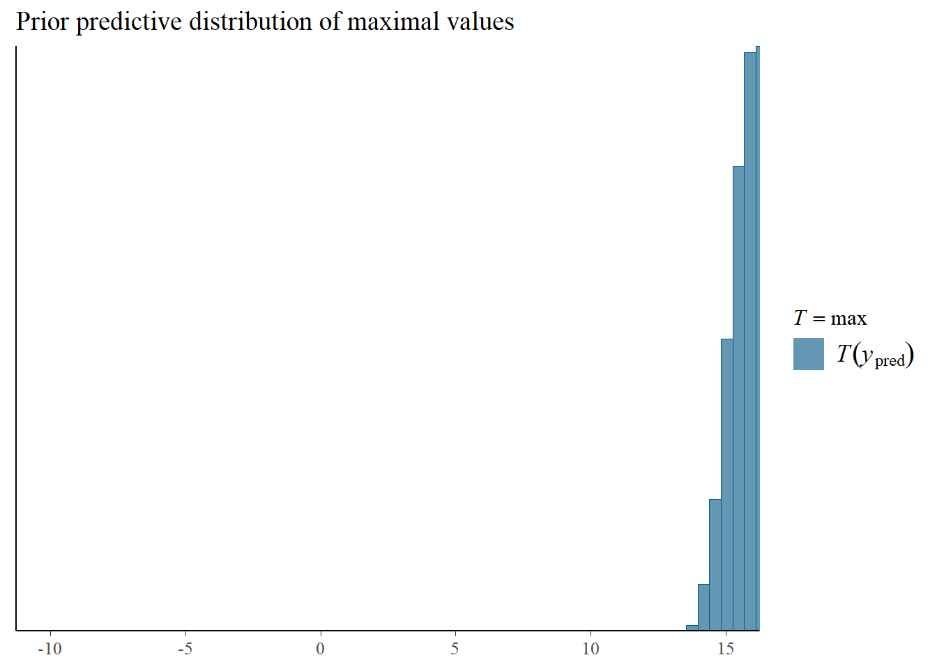
Let’s now also check whether the priors make sense
Model 8 - adding interactions
Possible interactions include:
CommAtt x Modality - Effort could increase differently across modalities, depending on whether concept is guessed on the first, second or third attempt. E.g., gesture might require more effort on initial attempt, but vocal require more effort in repeated attempt. This is interesting question and it would help disentangle the benfit of multimodality over unimodality (i.e., multimodal trials might be more effortful, but overal have less attempts). However, we already model effect of modality on effort, so maybe this is not top priority.
CommAtt x Expressibility - Higher expressibility should moderate the effect of repeated attempts, such that the increase in effort with each additional attempt is smaller (or bigger?) for more expressible concepts.This is not a priority for our analysis.
Modality × Expressibility_z - The influence of expressibility on effort could be modality-specific — perhaps effort increases less with expressibility in the combined modality. For our analysis, this is also not a priority (especially since expressibiliy has already modality encoded)
Familiarity x CommAtt - More familiar partners may guess faster (fewer attempts) and require less effort, but this effect could diminish over multiple attempts. For our analysis, this is not a priority,
Big5 × Modality or Big5 × CommAtt - More open/extraverted participants might maintain higher effort over attempts, or adjust more dynamically depending on the communicative channel. While not priority, it is an interesting question if we want to tap more into the inter-individual variability.
Let’s try CommAtt x Modality and Big5 x CommAtt
h1.m8 <-brm(Eff ~1+ CommAtt * Modality + Big5 * CommAtt + Familiarity + Expressibility_z + (1+ CommAtt | Participant) + (1+ CommAtt | Concept) + (1| TrialNumber_c), data = final_data,family =lognormal(),prior = priors_h1m7, # we keep the priors from previous modeliter =4000,cores =4)# Add criterions for later diagnosticsh1.m8 <-add_criterion(h1.m8, criterion =c("loo", "waic"))# Calculate also variance explained (R^2)h1.m8_R2 <-bayes_R2(h1.m8)# Save both as objectssaveRDS(h1.m8, here("09_Analysis_Modeling", "models", "h1.m8.rds"))saveRDS(h1.m8_R2, here("09_Analysis_Modeling", "models", "h1.m8_R2.rds"))beep(5)
# Coefficients remain mostly unchanged
# Since we did not really focused on the interactions during the simulation, we also don't have strong expectations here. But for the real data, there is a good reason to expect some meaningful values
plot(h1.m8)
# all goodplot(conditional_effects(h1.m8), points =TRUE)
# the effects all go in good direction# we can see here that combined modality remains moderated across all commatts# and also big5 seems to matter the most in the second attemptpp_check(h1.m8, type ="dens_overlay")
# the problem with predicting negative values remainspp_check(h1.m8, type ="error_scatter_avg")
So in terms of WAIC & LOO, interactions do not really add predictive power. This might be specific for the synthetic data, as we did not explicitly focused on the interaction coefficients there. At the same time, the difference of h1.m8 from h1.m6c is not so significant. For now, we stop here. With the full data, we will proceed with the same evaluation.
H2: Modelling
Now we can need to account also for our second hypothesis, namely
H2: A higher degree of misunderstanding will require a performer to engage in more effortful correction.
We operationalize degree of misunderstanding as a cosine similarity of performer’s target and guesser’s answer (PrevAn). The difficulty with our data structure is that PrevAn is a variable that has values only for second and third correction (i.e., there is no previous answer for the first performance). If we left it unchange, the model will eventually get rid of all NA values, which means we will loose the relationship between effort in second and first communicative attempt. To avoid this, we will create a new variable which we call Effort Change. We will simply calculate the change from effort in communicative attempt x to communicative attempt x+1. We will still loose communicative attempt 1, but the change that will be associated with CommAtt==2 already encapsulates the relationship towards this attempt.
Data wrangling I
# Calculate Effort Change (Difference)final_data_2 <- final_data %>%group_by(Participant, Concept) %>%mutate(Effort_1 = Eff[CommAtt ==1][1], # Effort for attempt 1Effort_2 = Eff[CommAtt ==2][1], # Effort for attempt 2Effort_3 = Eff[CommAtt ==3][1], # Effort for attempt 3Effort_Change_1_to_2 =case_when( CommAtt ==2&!is.na(Effort_1) ~ Eff - Effort_1, # Change from 1st to 2nd attemptTRUE~NA_real_ ),Effort_Change_2_to_3 =case_when( CommAtt ==3&!is.na(Effort_2) ~ Eff - Effort_2, # Change from 2nd to 3rd attemptTRUE~NA_real_ ) ) %>%ungroup()# Collide changes into a single columnfinal_data_2 <- final_data_2 %>%mutate(Effort_Change =coalesce(Effort_Change_1_to_2, Effort_Change_2_to_3) ) # Remove unnecessary columnsfinal_data_2 <-subset(final_data_2, select =-c(Effort_1, Effort_2, Effort_3, Effort_Change_1_to_2, Effort_Change_2_to_3)) # View the resulthead(final_data_2, n=15)
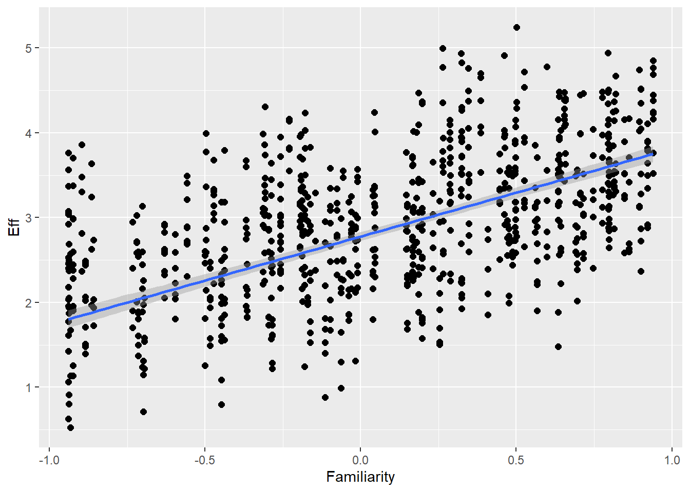
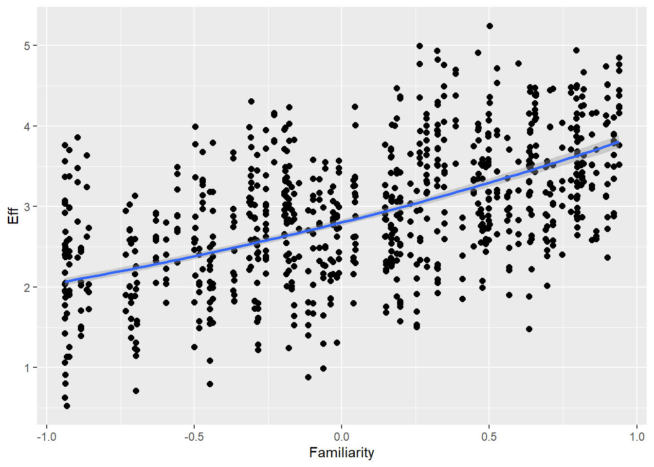
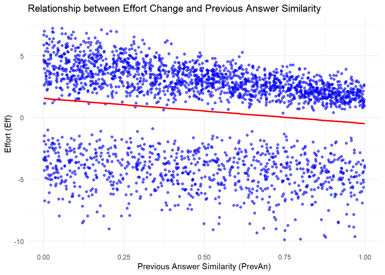
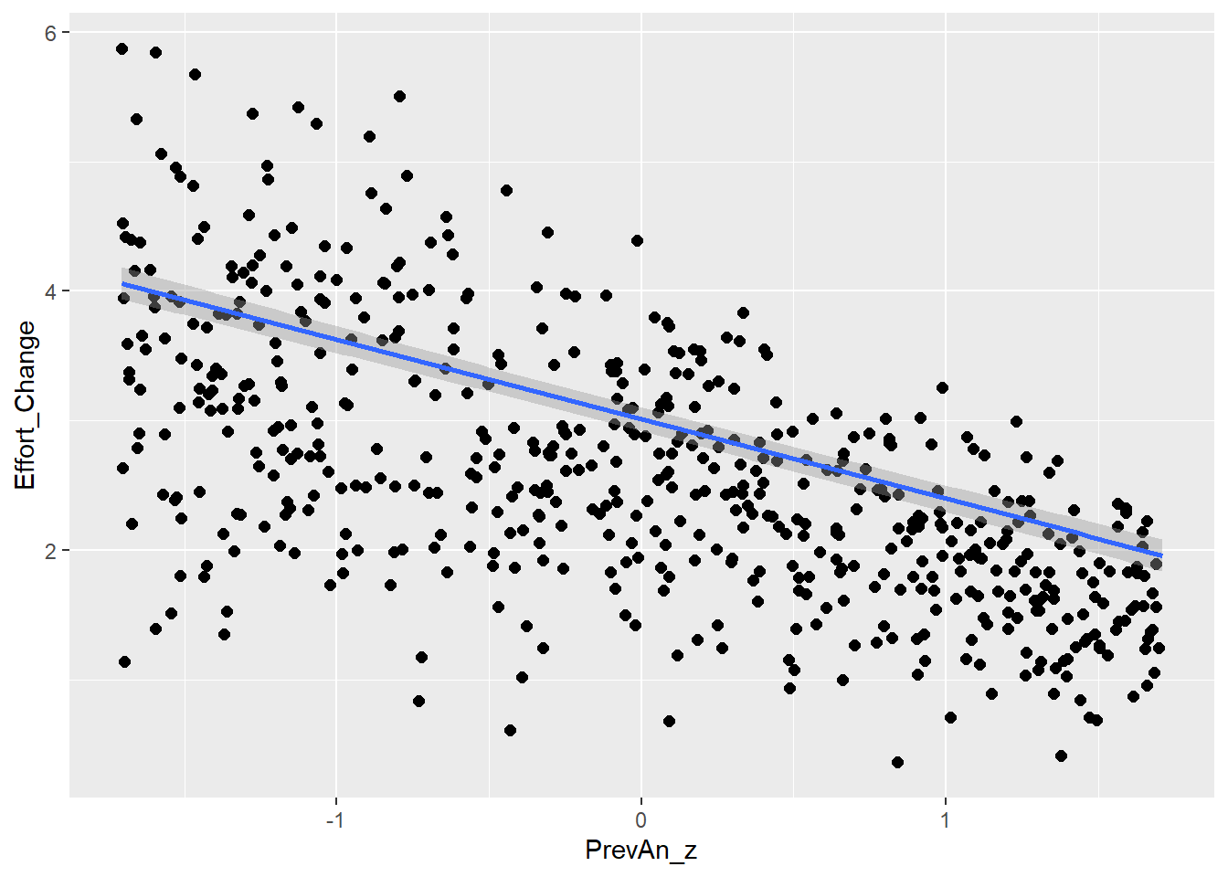
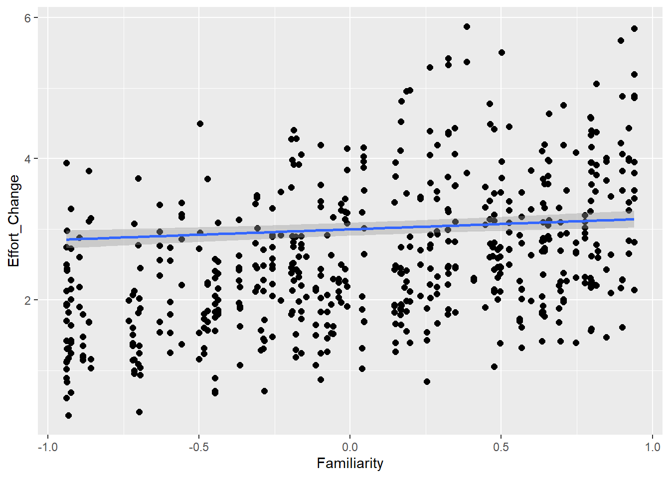
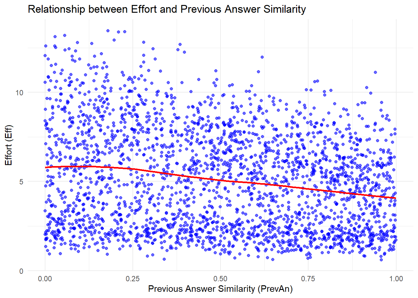
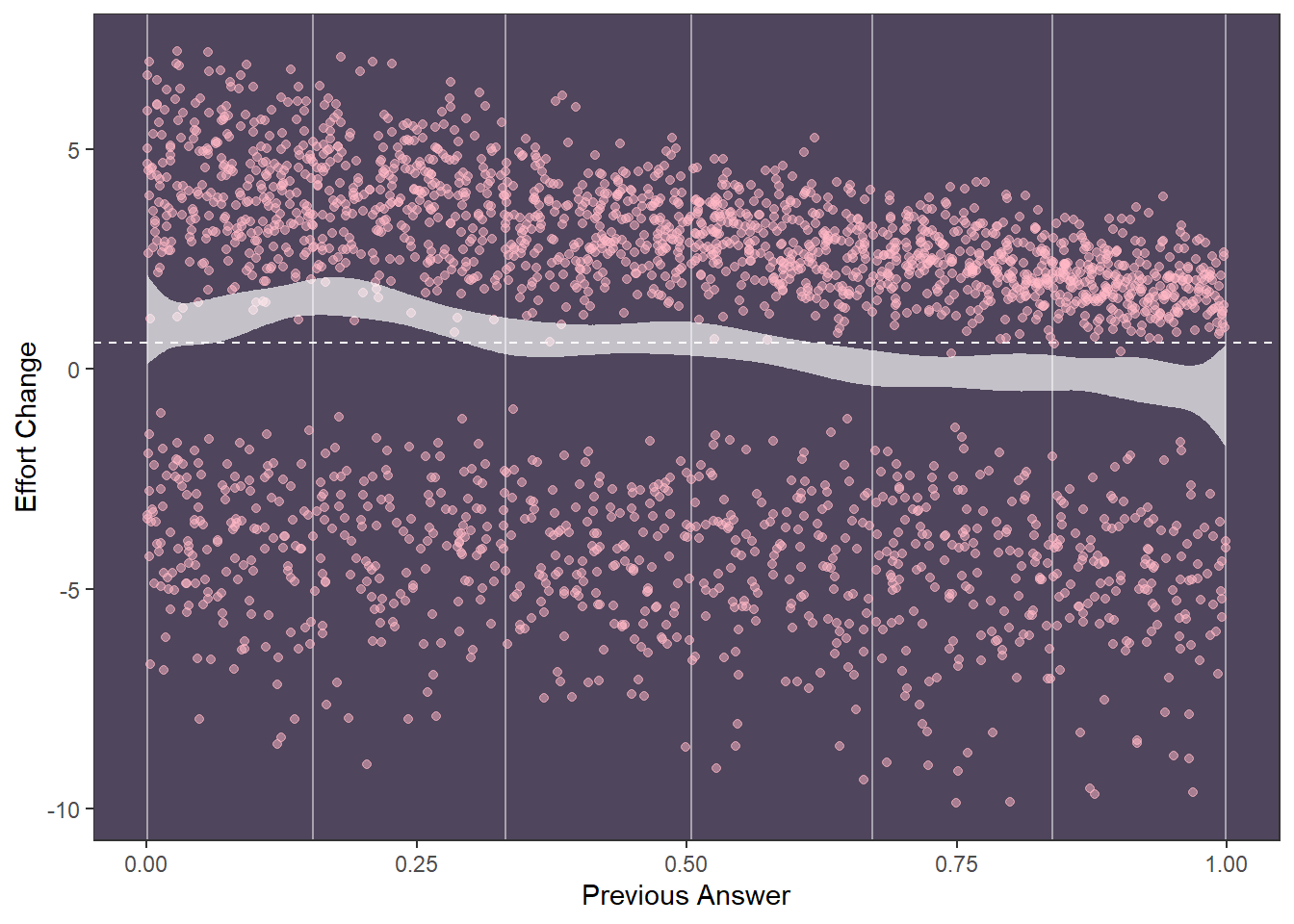
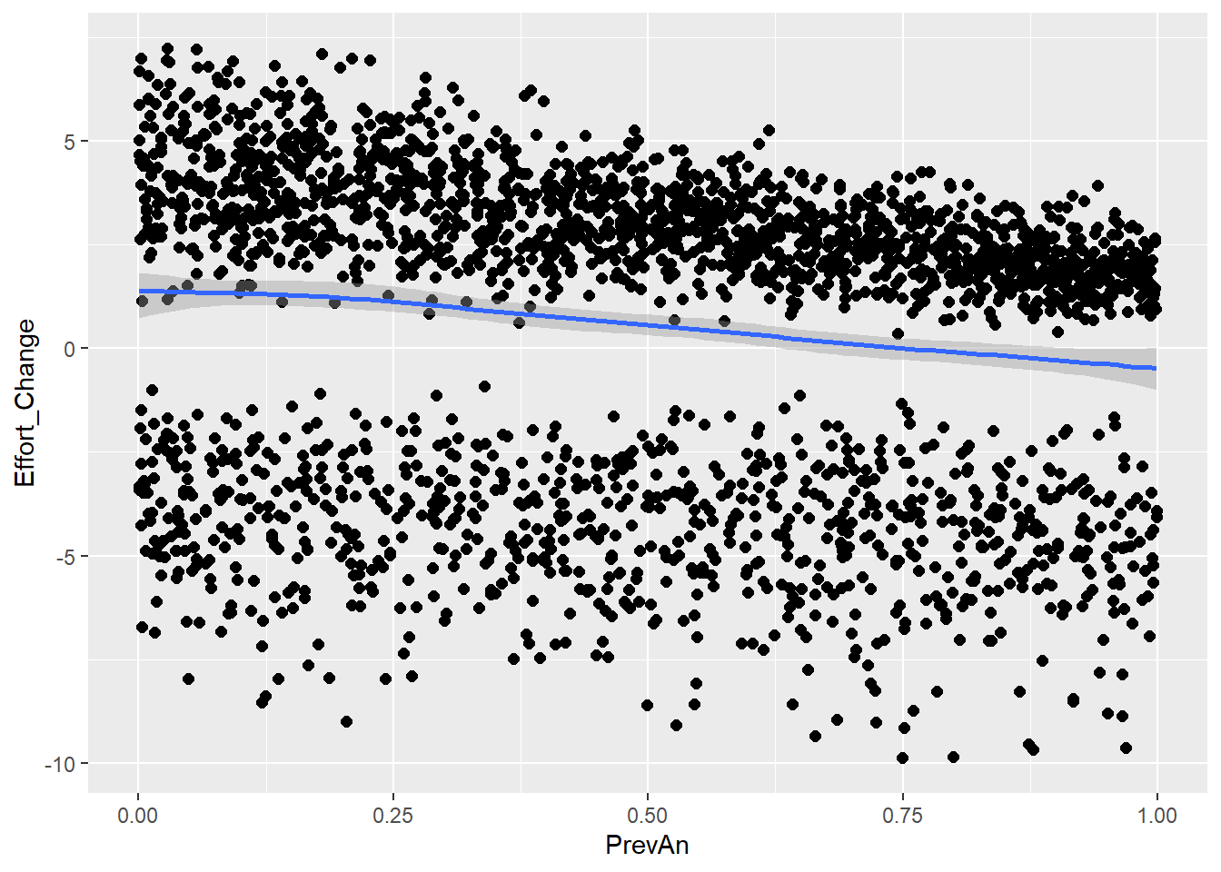
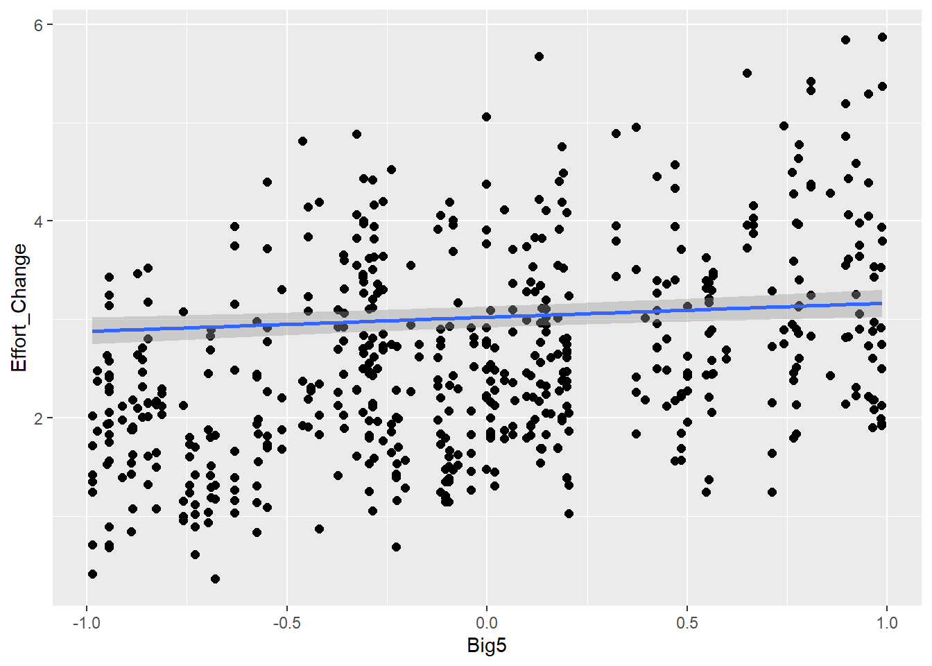
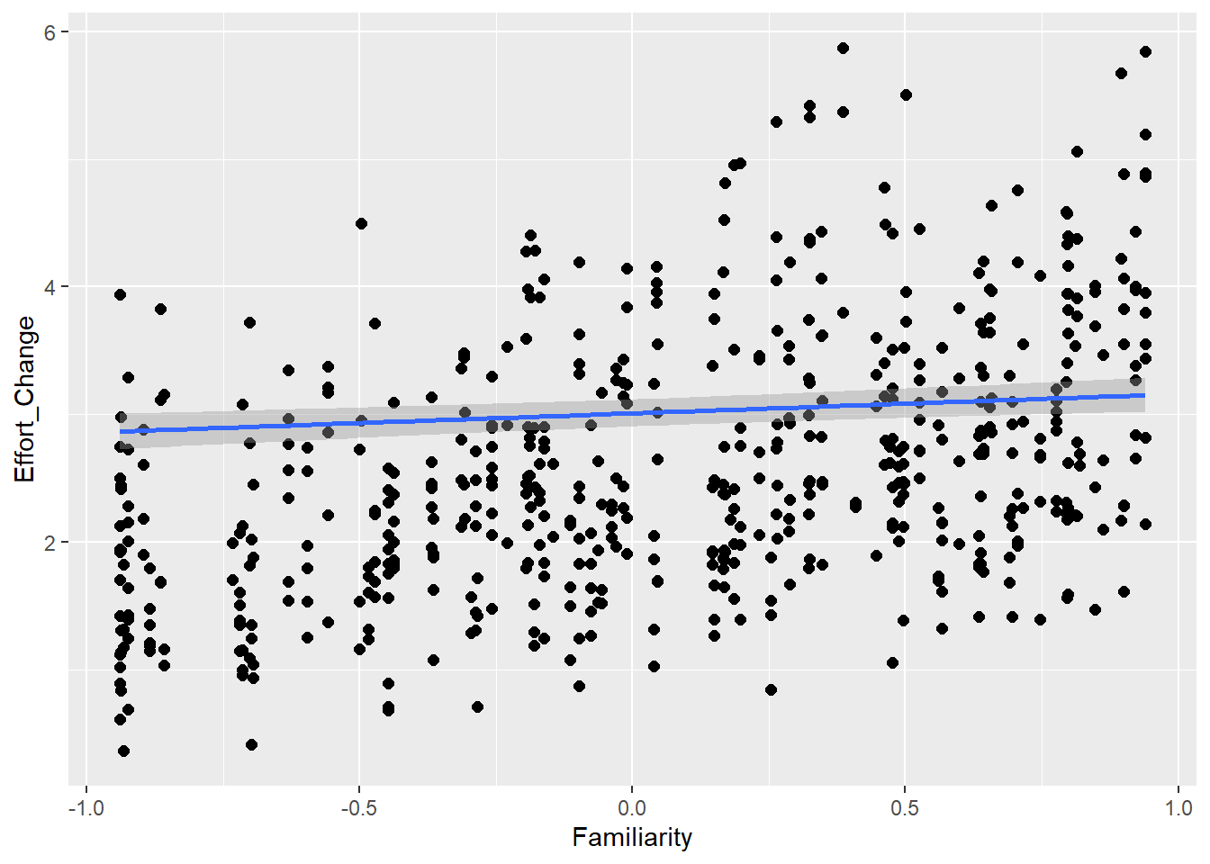
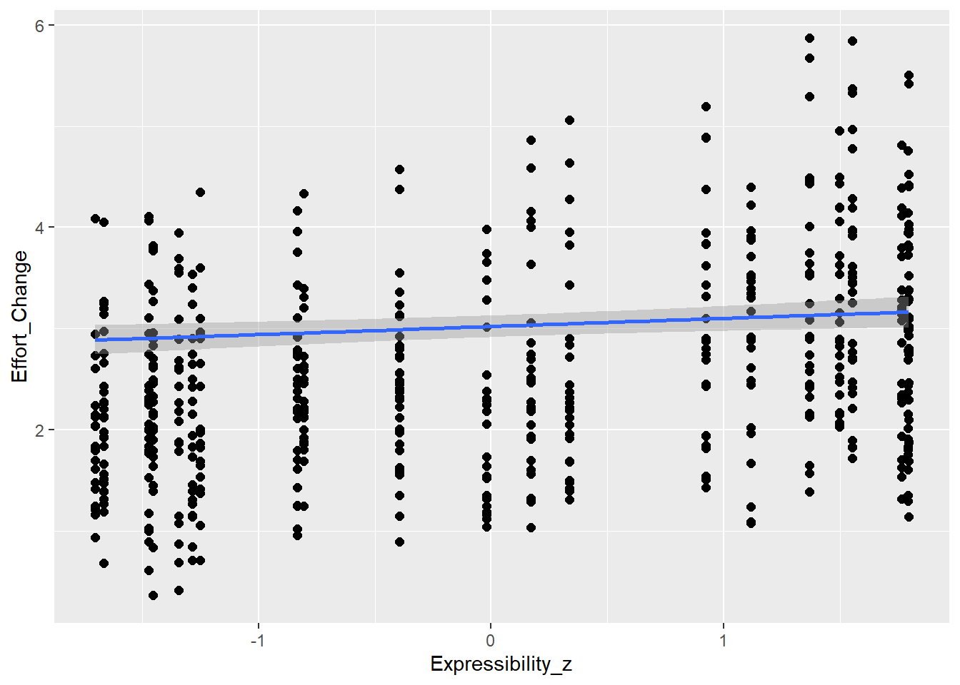
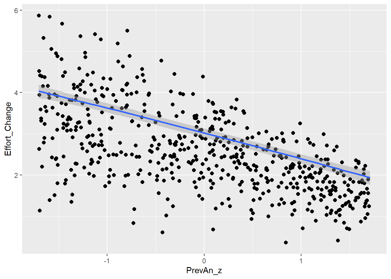
This is the relationship between effort and answer similarity (H2) as seen in the raw (synthetic) data
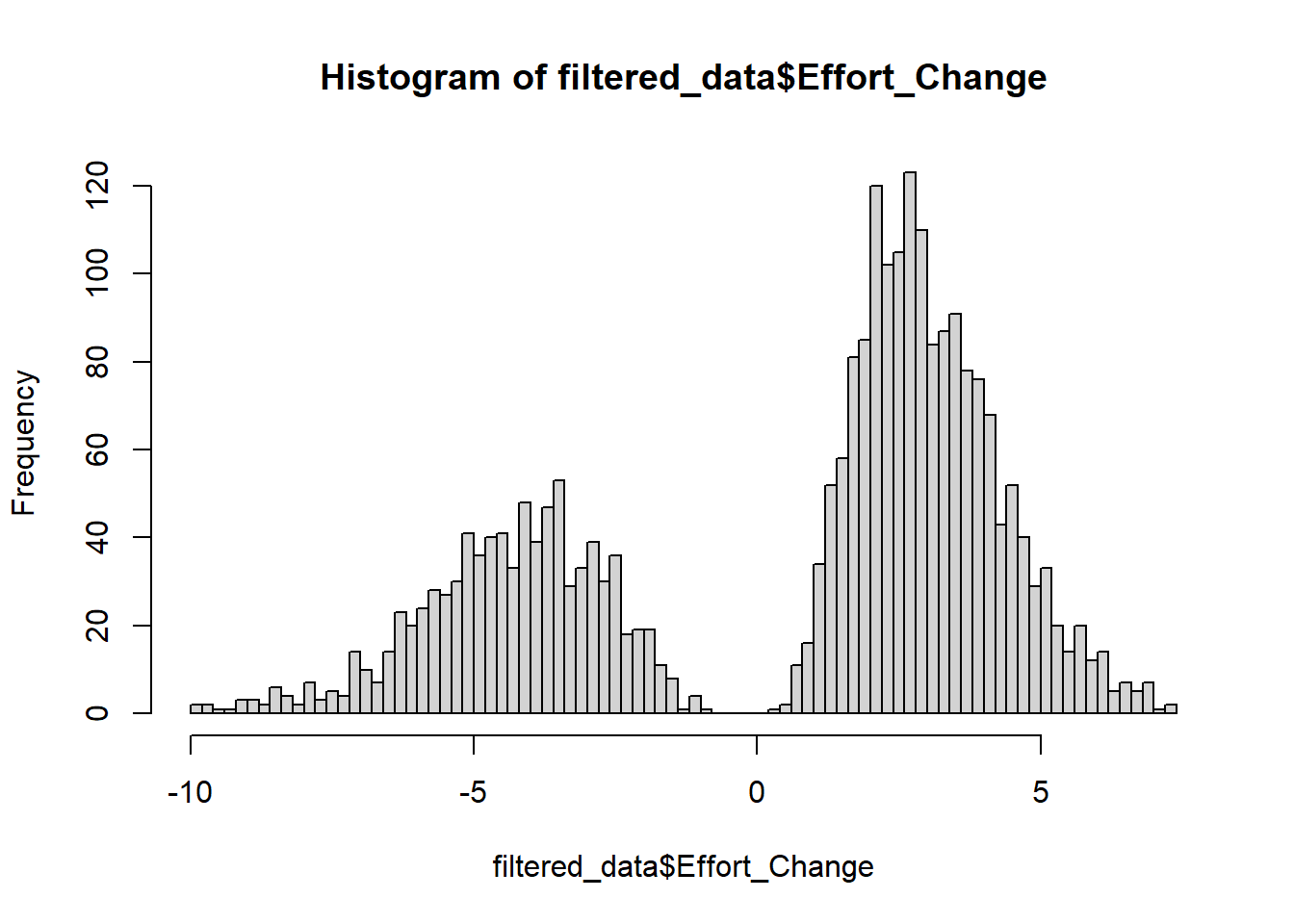
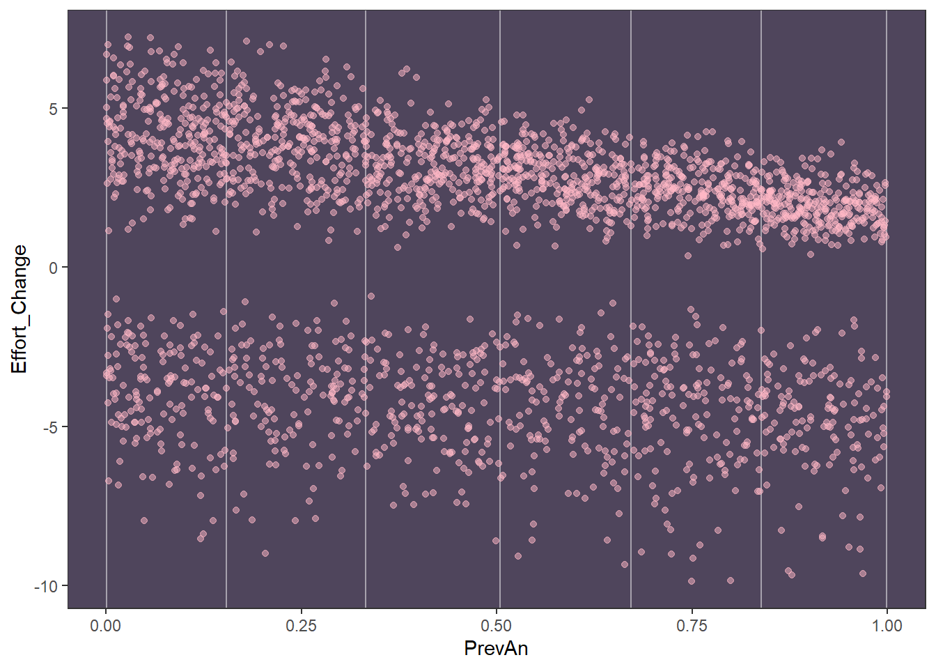
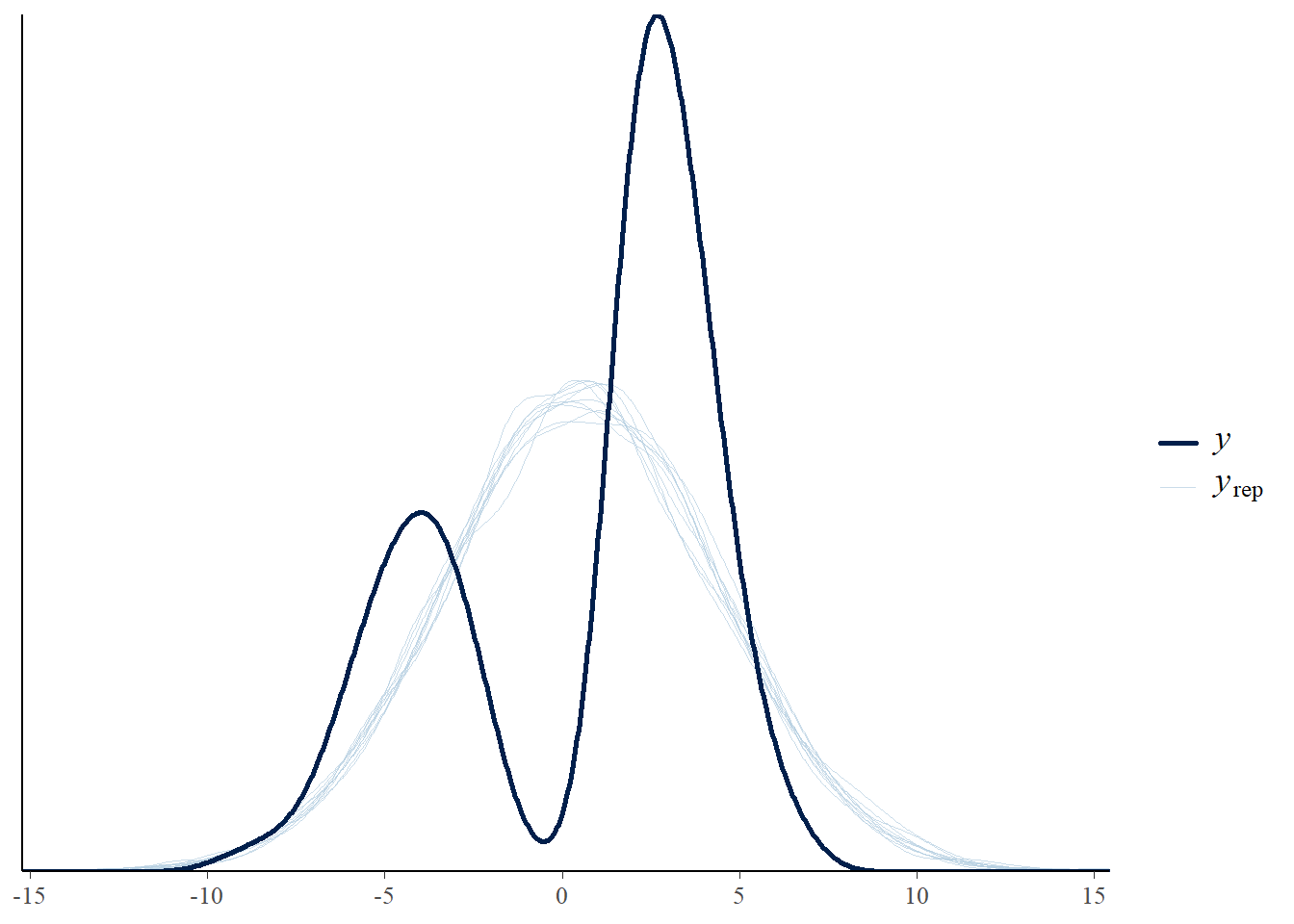
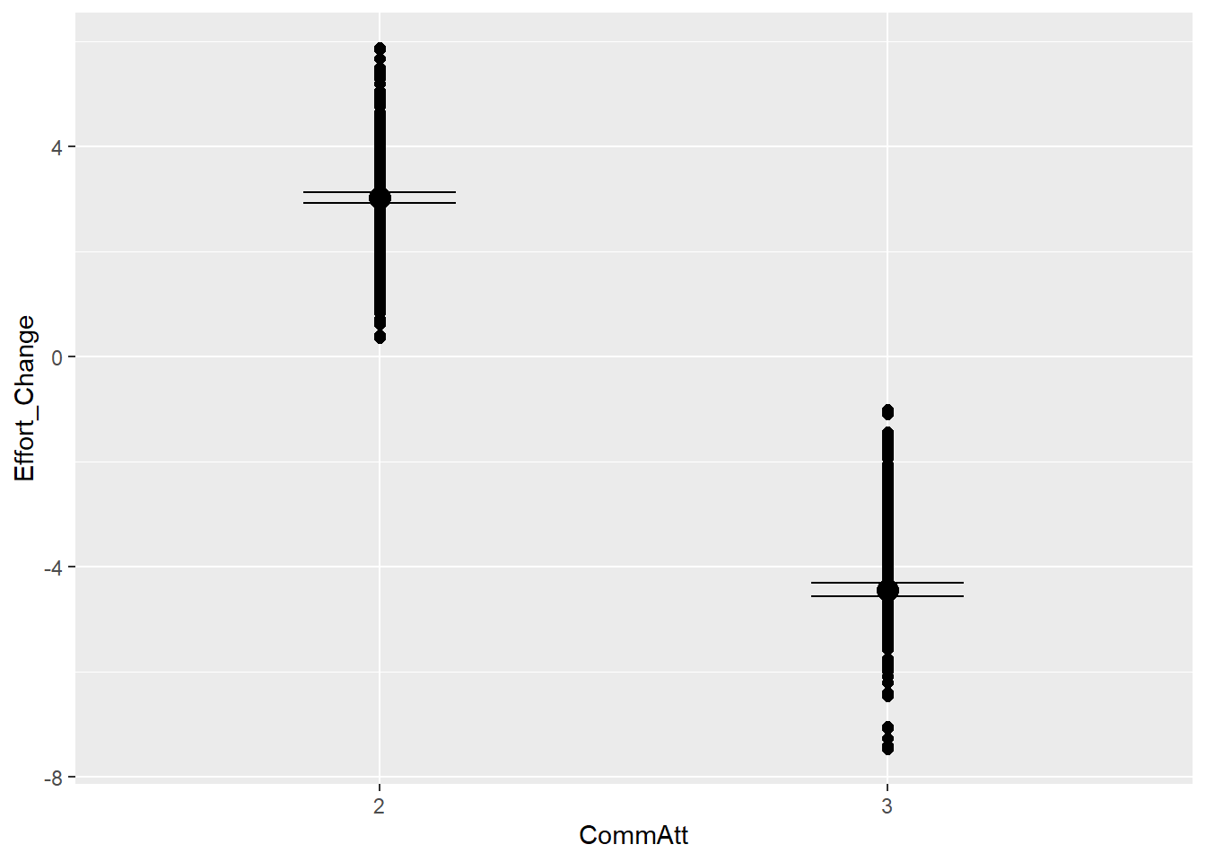
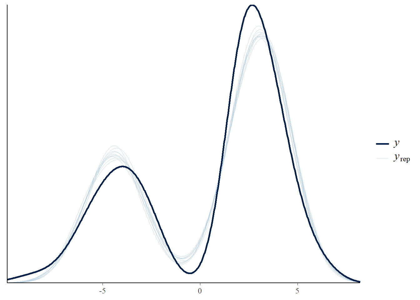
This is how effort change is distributed
So we will have to work with bimodal distribution, as we either have a decrease in effort or increase
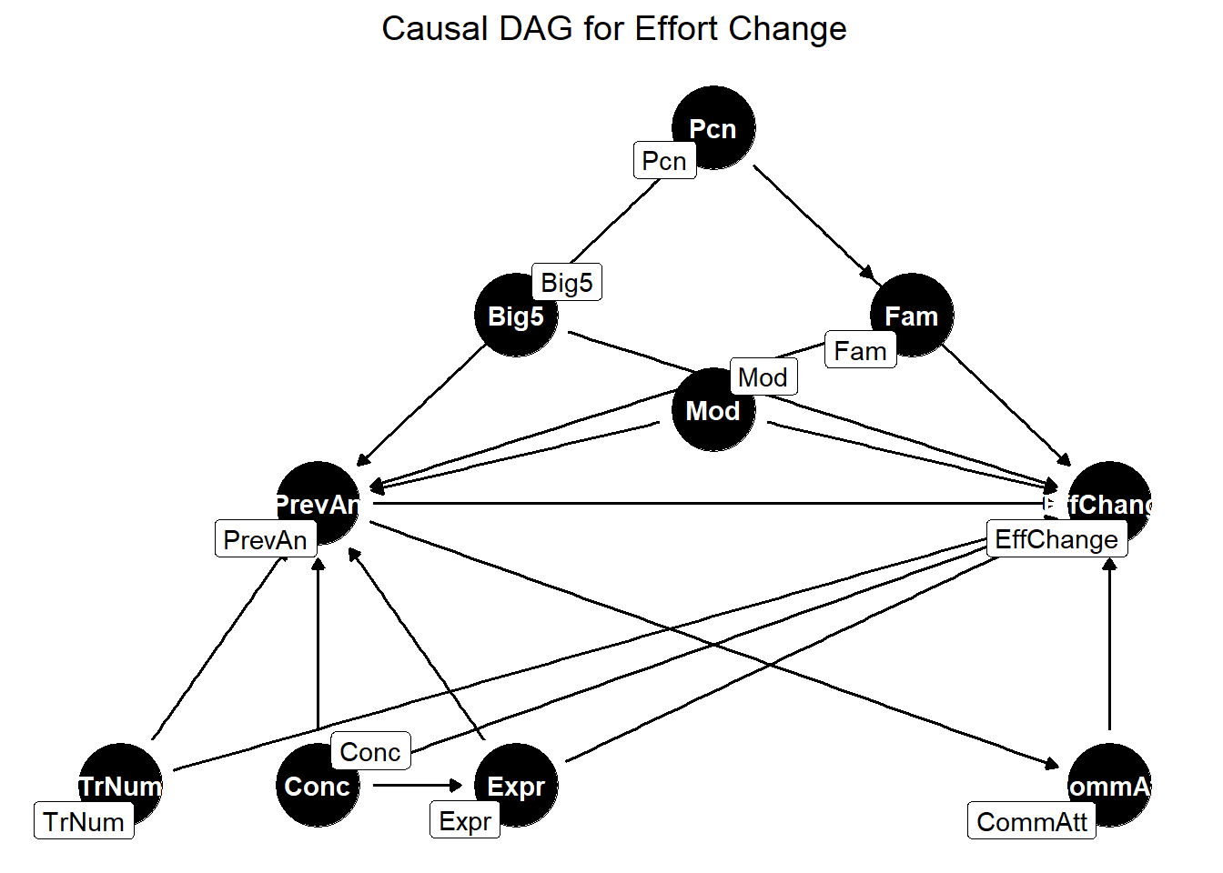
H2: Stating causal model
We now also need a new DAG. Essentially, what we said will influence CommAtt in H1, will now also influence PrevAn because they are tightly related. For instance, more extroverted people can be expected to be better guessers, therefore the similarity of the previous answer will be higher.
The adjustment set is identical to the one of H1. Note that we are here omitting arrows going from all these variables to ComAtt. Since PrevAn affects CommAtt, and not the other way, we do not need to block this path to avoid confounds. However, if we want to asses direct effect of PrevAn on EffChange, we have to add CommAtt to the model as well.
H2: Modelling
Converting columns to factors
filtered_data$CommAtt <-as.factor(filtered_data$CommAtt)filtered_data$CommAtt <-droplevels(filtered_data$CommAtt) # commatt1 still remains as a levelfiltered_data$CommAtt <-as.factor(filtered_data$CommAtt) # redo againfiltered_data$Modality <-as.factor(filtered_data$Modality)filtered_data$Participant <-as.factor(filtered_data$Participant)filtered_data$Concept <-as.factor(filtered_data$Concept)filtered_data$TrialNumber <-as.numeric(filtered_data$TrialNumber) # Ensure TrialNumber is numeric
 Family: gaussian
  Links: mu = identity; sigma = identity
Formula: Effort_Change ~ 1 + PrevAn_z + CommAtt + Familiarity + Big5 + Expressibility_z + TrialNumber_c + Modality + (1 | Participant) + (1 | Concept)
   Data: filtered_data (Number of observations: 2556)
  Draws: 4 chains, each with iter = 4000; warmup = 2000; thin = 1;
         total post-warmup draws = 8000

Multilevel Hyperparameters:
~Concept (Number of levels: 21)
              Estimate Est.Error l-95% CI u-95% CI Rhat Bulk_ESS Tail_ESS
sd(Intercept)     0.03      0.02     0.00     0.09 1.00     5564     4490

~Participant (Number of levels: 120)
              Estimate Est.Error l-95% CI u-95% CI Rhat Bulk_ESS Tail_ESS
sd(Intercept)     0.02      0.02     0.00     0.07 1.00     6328     4353

Regression Coefficients:
                 Estimate Est.Error l-95% CI u-95% CI Rhat Bulk_ESS Tail_ESS
Intercept           -0.66      0.03    -0.71    -0.60 1.00    13909     5911
PrevAn_z            -0.62      0.02    -0.66    -0.57 1.00    17850     5508
CommAtt1             3.73      0.03     3.68     3.79 1.00    19981     5855
Familiarity          0.15      0.05     0.06     0.24 1.00    16619     5695
Big5                 0.14      0.04     0.06     0.23 1.00    16358     5795
Expressibility_z     0.08      0.03     0.02     0.13 1.00    17823     5427
TrialNumber_c        0.00      0.00    -0.00     0.01 1.00    11346     5008
Modality1           -0.14      0.07    -0.28     0.00 1.00    13812     6660
Modality2            0.01      0.07    -0.12     0.15 1.00    11997     6265

Further Distributional Parameters:
      Estimate Est.Error l-95% CI u-95% CI Rhat Bulk_ESS Tail_ESS
sigma     1.25      0.02     1.21     1.29 1.00    19597     4922

Draws were sampled using sampling(NUTS). For each parameter, Bulk_ESS
and Tail_ESS are effective sample size measures, and Rhat is the potential
scale reduction factor on split chains (at convergence, Rhat = 1).
# coefficients seem quite conservative, even for PrevAn (but remember, it's z-scored)
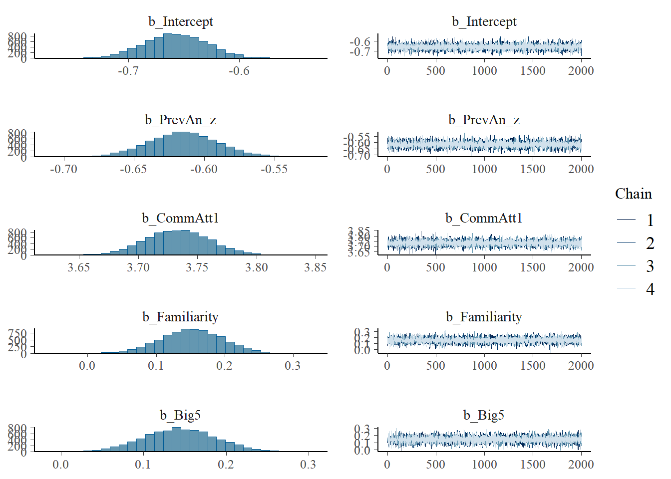
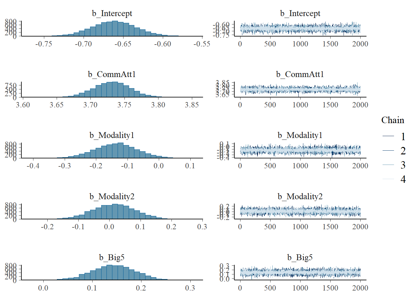
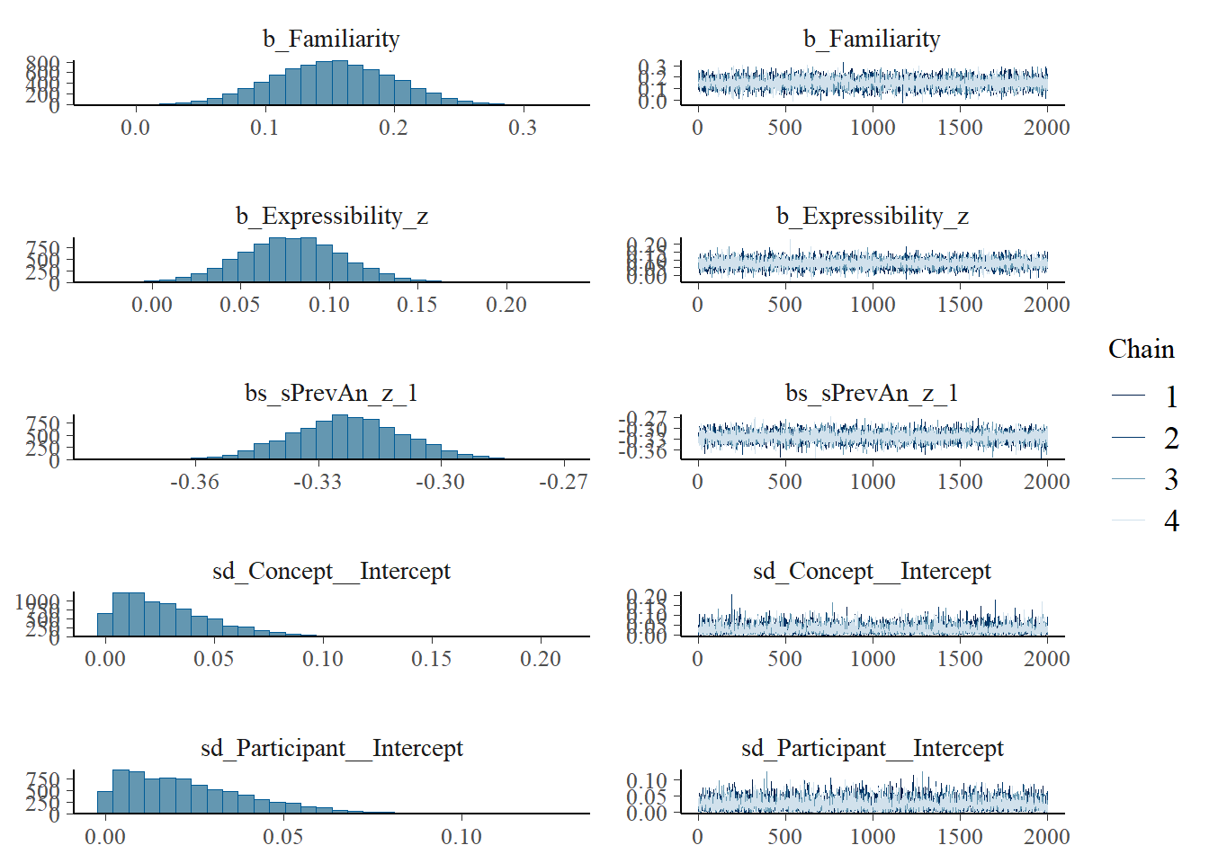
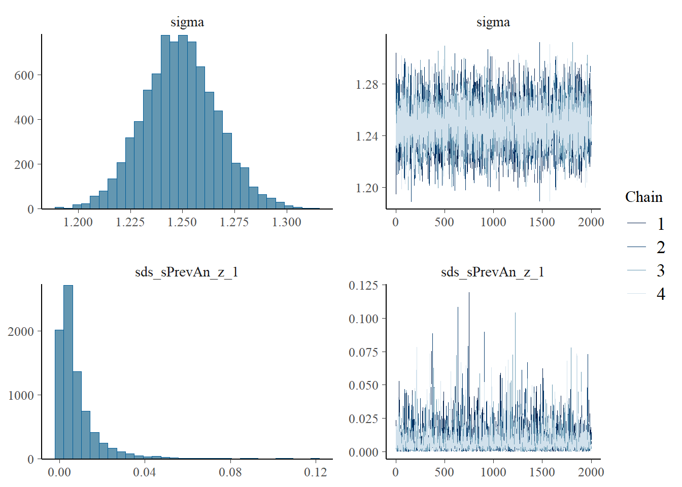
plot(h2.m1)
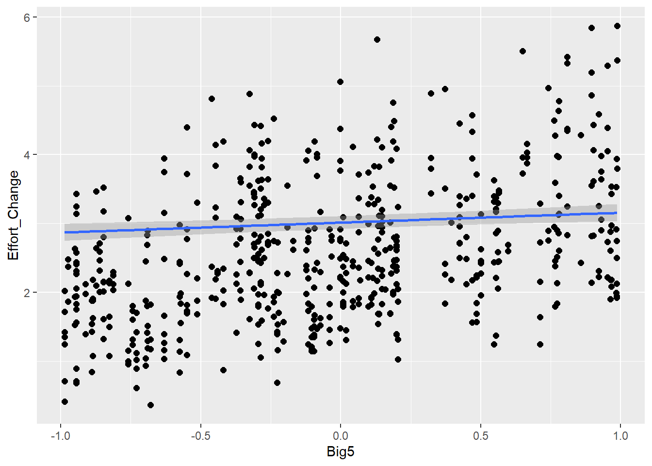
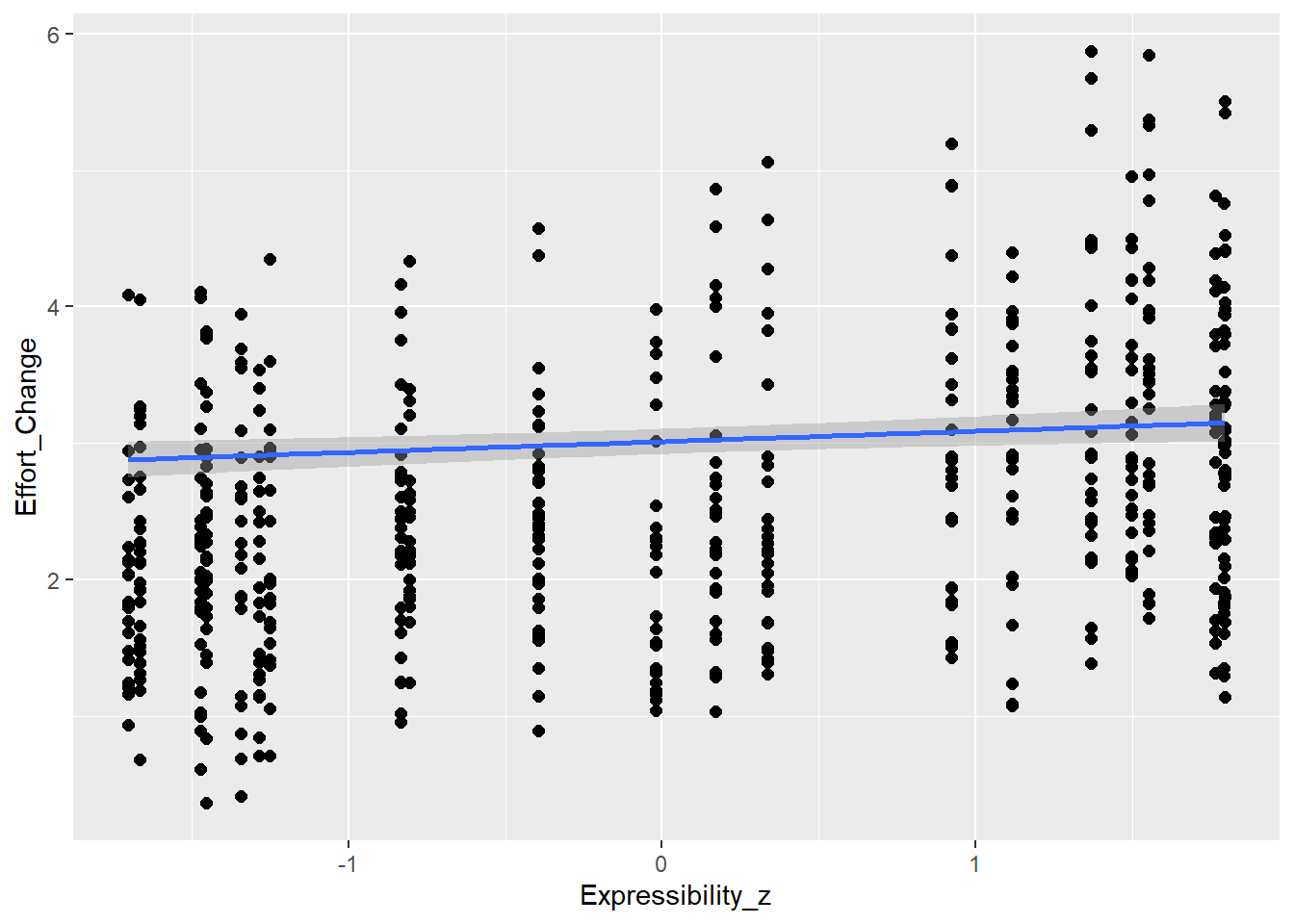
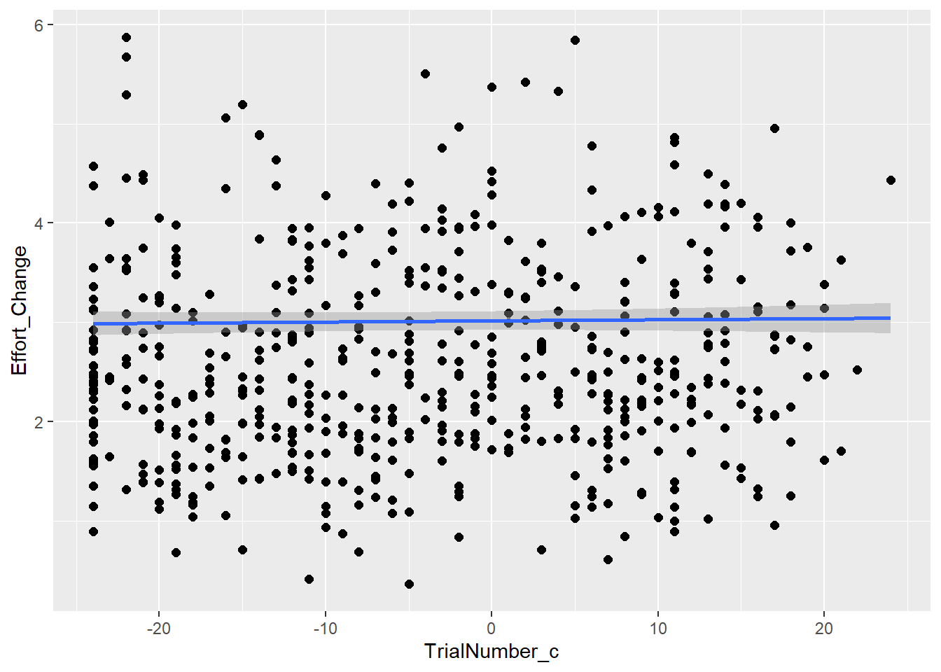
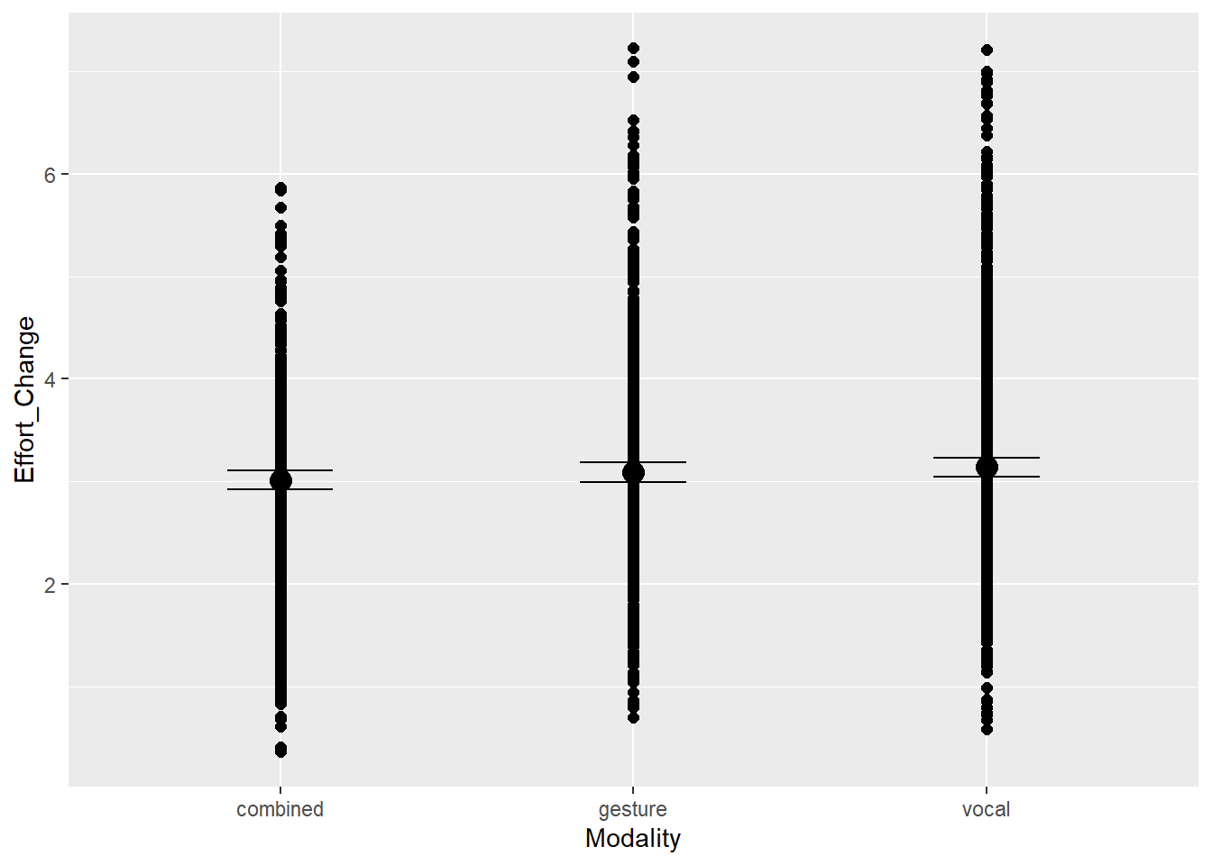
# all looks okplot(conditional_effects(h2.m1), points =TRUE)
# the main effect seems ok, the rest of the predictors does not show nothing (maybe because of the transformation we lost the relations between them and the effort)pp_check(h2.m1, type ="dens_overlay")
# this looks quite okay-ishpp_check(h2.m1, type ="error_scatter_avg")
# so there seems to be quite high residual errorh2.m1_R2
We see two modes in the distribution of the predictor. While Gaussian family seems to deal with it well, we could also consider model with mixture of two Gaussian distributions. This will allow each mode to have their own mean and variance. With effort change being distributed over positive as well as negative values, lognormal distribution is not applicable.
Importantly, there are some diagnostics we should be cautious about - the relationship between predicted values and residual error is quite correlated.
Also notice the high explained variance indicated by R^2. In real case, this would be almost pointing to over-fitting issues. However, we created synthetic data that does not contain as much noise as we can expect from the real data, so it is quite likely that if we simply used all predictors we know to cause a variance here, we might be explaining most of the variation. It is quite likely this will not be the case for real data.
Splines 1 - fitting b-splines
In the previous model for H1, we were able to spot possible non-linear trends by contrast coding of the communicative attempts whereby each level was defined relative to the two remaining. Now, we are dealing with situation where both outcome variable and the main predictor are continuous variable. Also here we might expect nonlinear patterns in their relationship. For instance, it might be the case that for answers that are completely off, people do not feel motivated to put in more effort, and some kind of sensible ‘threshold’ needs to be reached for the effort to increase to resolve misunderstanding, and then again decrease when the answer is very similar.
We will use a combination of B-splines and Bayesian GAMs to prepare some models and try them fit to the synthetic data. However, note that we currently do not expect any non-linearity as we have not coded any within the simulation, as seen in the following plot fitted with loess method.
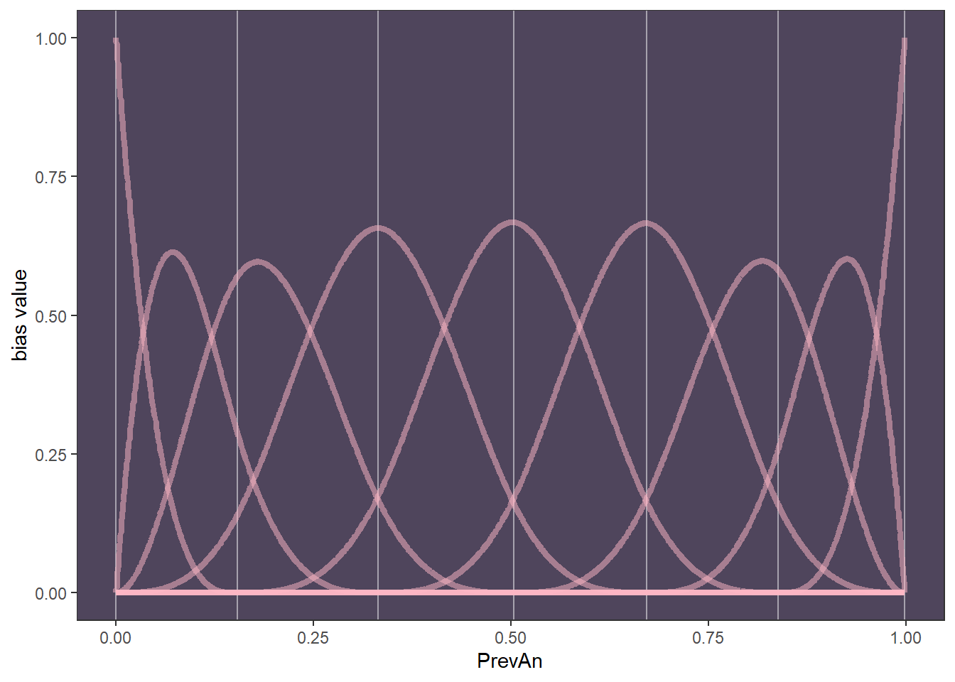
B-splines allow to build up wiggly functions from more simple components which are called ‘basis functions’ (B). They divide a full range of predictor into parts and assign a parameter to each part. The parameters are gradually turned on and off in a way that makes their sum into a curve. Unlike polynomial regression, b-splines do not transform predictor, but they invent a series of new synthetic predictor variables. Each of them then exists only to gradually turn a specific parameter on and off within a specific range of the real predictor variable. Each of these synthetic variables is called a basis function B. See more in Richard McElreath’s Statistical Rethinking (McElreath 2018).
We are using the code from Solomon Kurz’s adaptation of this book.
# Get rid of NAs in the predictord <- final_data_2 %>%drop_na(PrevAn)# And convert all that is necessary to factor/numericald$CommAtt <-as.factor(d$CommAtt)d$Modality <-as.factor(d$Modality)d$Participant <-as.factor(d$Participant)d$Concept <-as.factor(d$Concept)d$TrialNumber <-as.numeric(d$TrialNumber)
Now we need to specify knots that function as pivots for number of different basis functions. The B variable then tells you which knot you are close to.
The B matrix is now a matrix column which contains the same number of rows as the others, but has also 9 columns within that columns. Each of them correspond to one synthetic B variable.
We can now use this matrix to fit our model
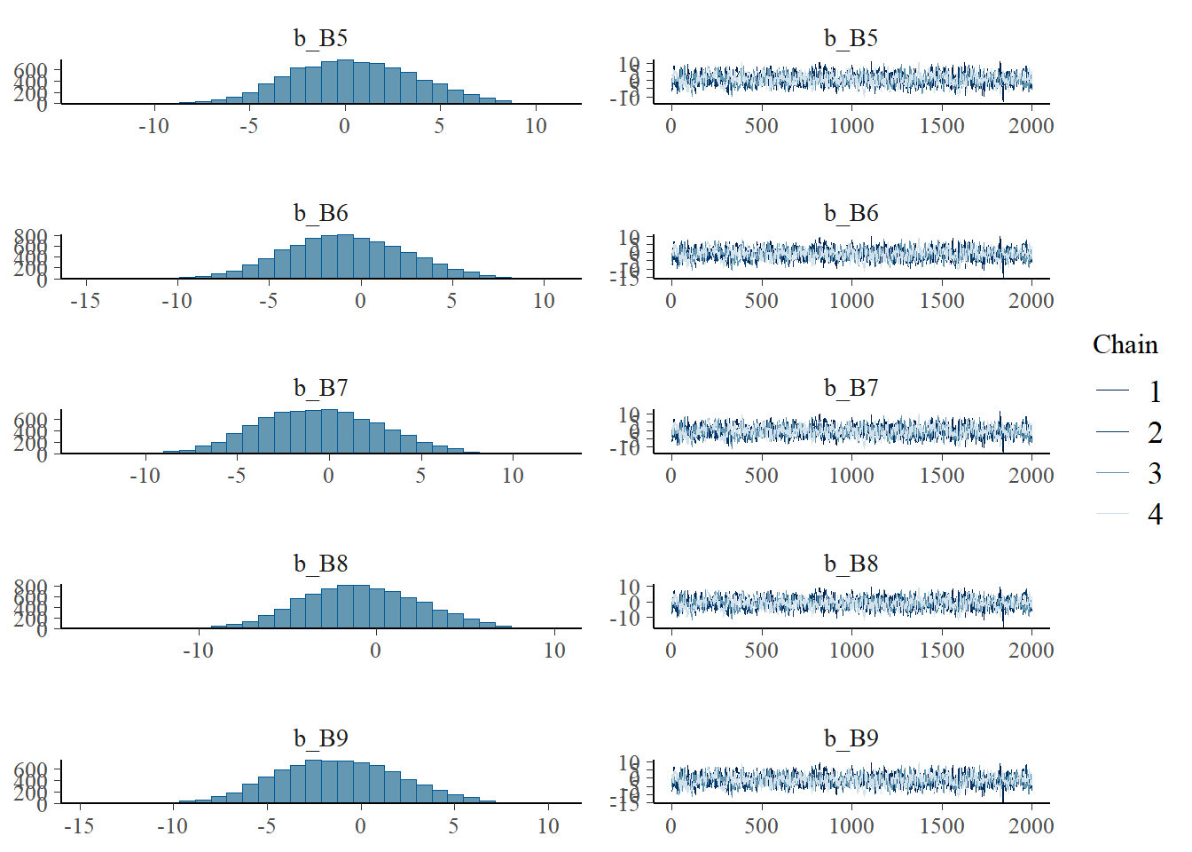
h2.s1 <-brm(data = d2,family = gaussian, Effort_Change ~1+ B,prior =c(prior(normal(100, 10), class = Intercept),prior(normal(0, 10), class = b),prior(exponential(1), class = sigma)),iter =4000, warmup =2000, chains =4, cores =4,seed =4)# Add criterions for later diagnosticsh2.s1 <-add_criterion(h2.s1, criterion =c("loo", "waic"))# Calculate also variance explained (R^2)h2.s1_R2 <-bayes_R2(h2.s1)# Save both as objectssaveRDS(h2.s1, here("09_Analysis_Modeling", "models", "h2.s1.rds"))saveRDS(h2.s1_R2, here("09_Analysis_Modeling", "models", "h2.s1_R2.rds"))beep(5)
Family: gaussian
Links: mu = identity; sigma = identity
Formula: Effort_Change ~ 1 + B
Data: d2 (Number of observations: 2556)
Draws: 4 chains, each with iter = 4000; warmup = 2000; thin = 1;
total post-warmup draws = 8000
Regression Coefficients:
Estimate Est.Error l-95% CI u-95% CI Rhat Bulk_ESS Tail_ESS
Intercept 0.60 3.29 -5.87 6.72 1.00 1022 1772
B1 0.54 3.32 -5.66 7.08 1.00 1043 1951
B2 0.15 3.34 -6.13 6.70 1.00 1044 1856
B3 1.83 3.34 -4.47 8.44 1.00 1057 1901
B4 -0.33 3.32 -6.66 6.19 1.00 1042 1844
B5 0.42 3.31 -5.80 6.88 1.00 1041 1814
B6 -0.81 3.31 -7.00 5.71 1.00 1036 1880
B7 -0.57 3.33 -6.88 5.95 1.00 1049 1780
B8 -0.89 3.34 -7.14 5.67 1.00 1067 2043
B9 -1.21 3.32 -7.50 5.35 1.00 1039 1822
Further Distributional Parameters:
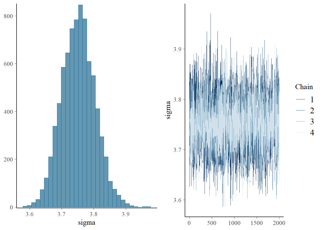
Estimate Est.Error l-95% CI u-95% CI Rhat Bulk_ESS Tail_ESS
sigma 3.75 0.05 3.65 3.85 1.00 4696 4264
Draws were sampled using sampling(NUTS). For each parameter, Bulk_ESS
and Tail_ESS are effective sample size measures, and Rhat is the potential
scale reduction factor on split chains (at convergence, Rhat = 1).
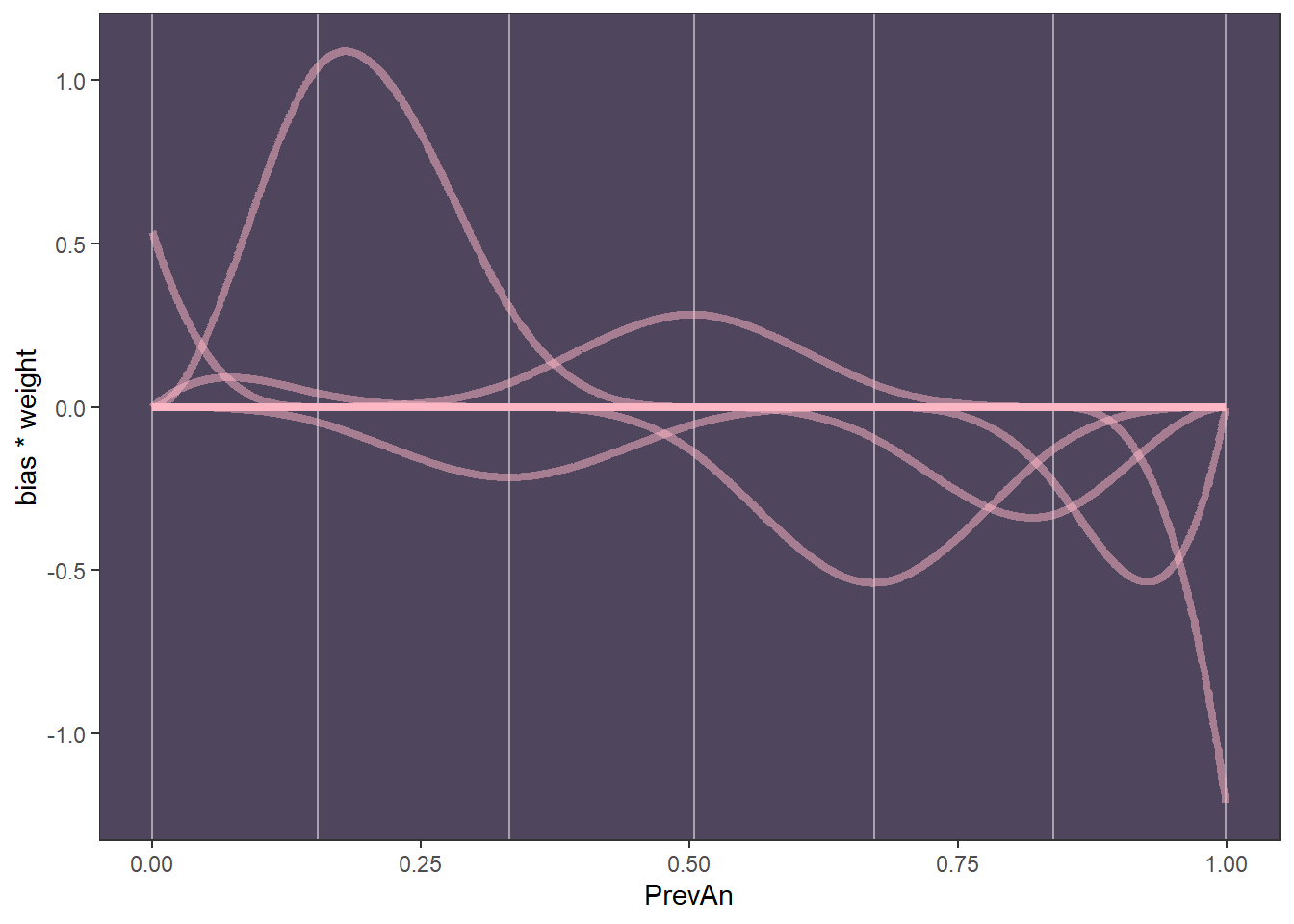
It’s a bit difficult to see what is going on so let’s just plot it
Now with the predictor
So as expected, we see quite linear decrease similar to our previous models
Now let’s check some diagnostics
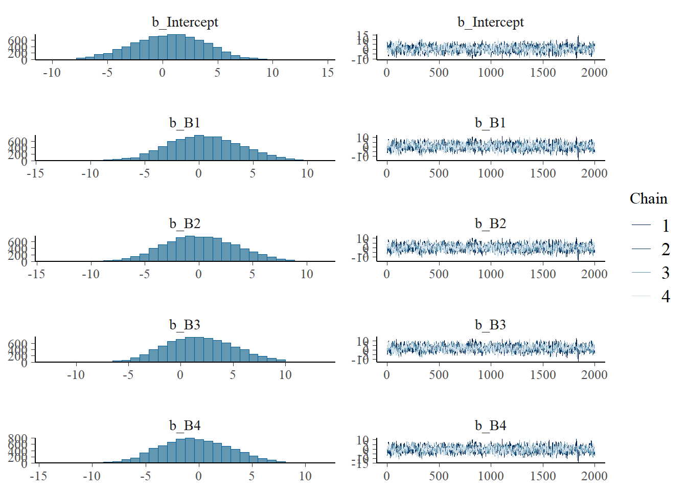
plot(h2.s1)
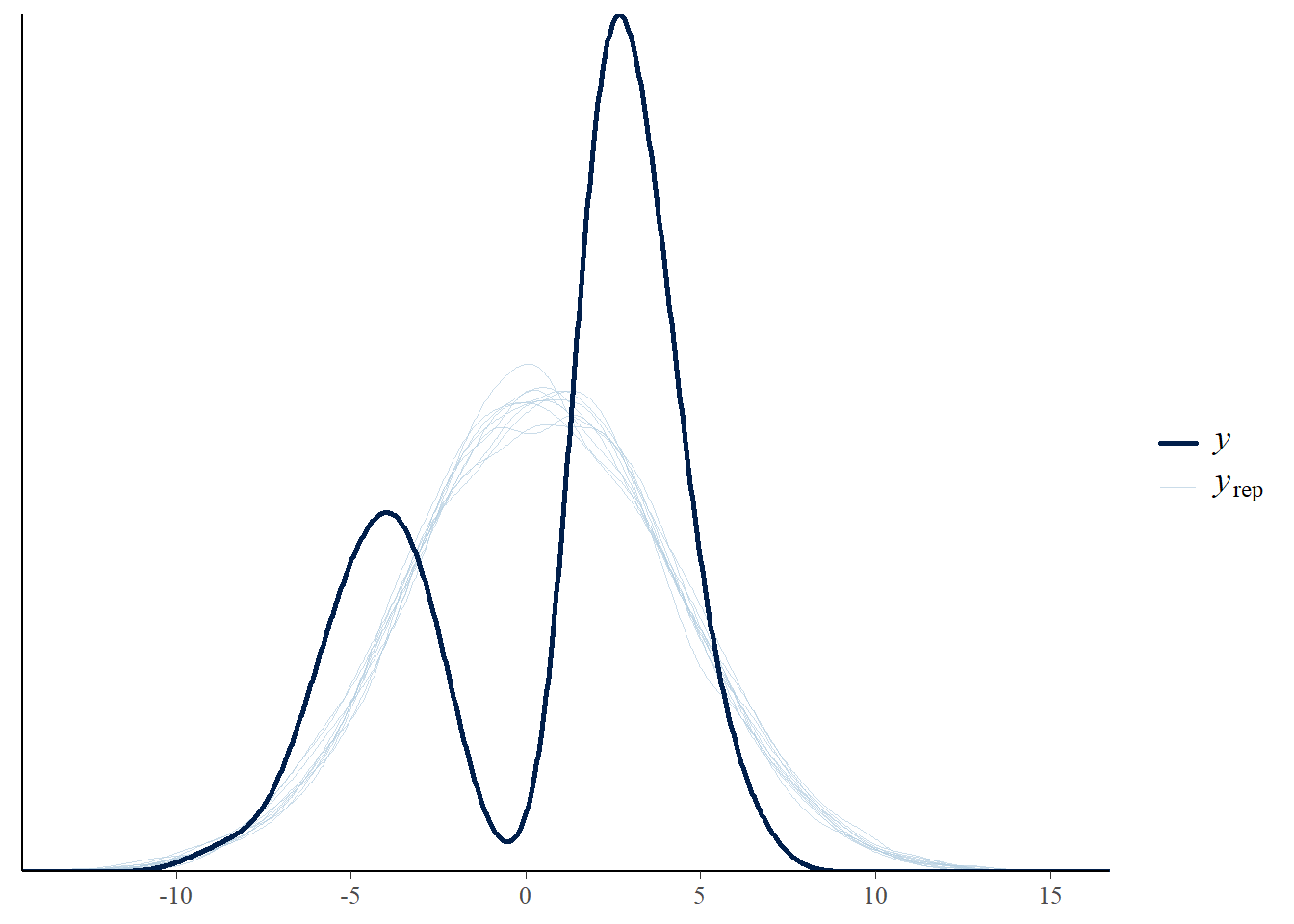
# looks goodpp_check(h2.s1, type ="dens_overlay")
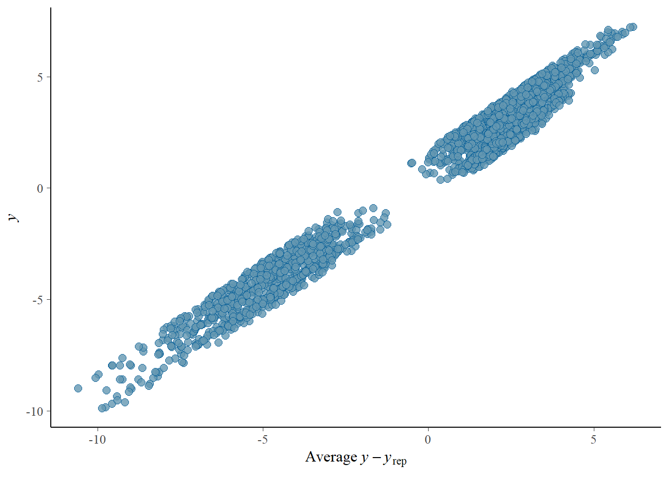
# because we used only main predictor, we can see quite a bad result of the posterior predictive distribution, but we will work on thatpp_check(h2.s1, type ="error_scatter_avg")
# high residual error for both low and high valuesh2.s1_R2
Now we will use a different workflow, using smooth functions with brms package. Brms allow for non-linear models by borrowing functions from mgcv package (Wood 2017)
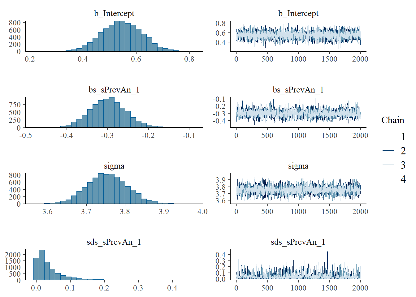
This is how priors should look like for one of these functions
# now the ffect of PrevAn looks a bit different because we are back to using z-scored versionpp_check(h2.s3, type ="dens_overlay")
# looks ok but the ppd undershoots the low values and overshoot the high values, similar to the linear regressionpp_check(h2.s3, type ="error_scatter_avg")
Effective sample size tells how many independent samples the model has effectively drawn from the PD. Low ESS suggests autocorrelation (i.e., sample explores one part of posterior), while high ESS means good mix
# Extract n_eff values for each modelneff_ratio_list <-lapply(model_list, function(model) { neff_values <-neff_ratio(model) # Here we calculate ratio (not the raw number of effective samples)data.frame(model =deparse(substitute(model)), min_neff =min(neff_values), max_neff =max(neff_values),mean_neff =mean(neff_values))})# Combine and inspectdo.call(rbind, neff_ratio_list)
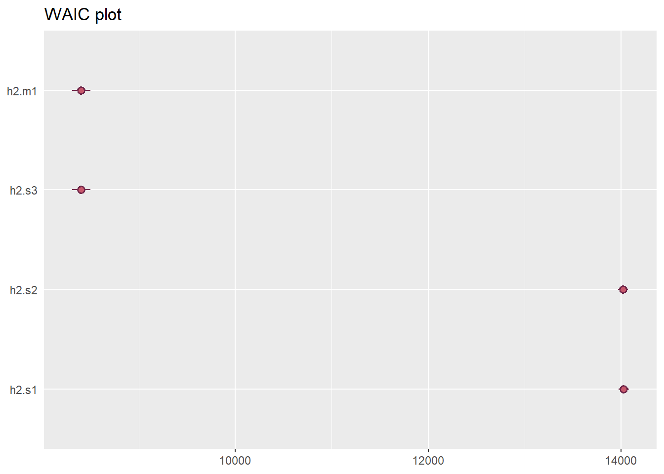
They all look good expect the very first non-linear model h2.s1 which is quite expectable since we used only main predictor. Linear regression model and GAMs model have highest ESS.
For the synthetic data, GAMs are probably adding unnecessary complexity as we are not gaining much more explanatory power. However, we leave it open whether linear or non-linear models will be better suited for the real data, following this pipeline.
Adding priors
Similarly to H1, we will also set mildly informative priors. Let’s check what priors have been selected as default for h2.s3
# Print priorsprior_summary(h2.s3)
prior class coef group
(flat) b
(flat) b Big5
(flat) b CommAtt1
(flat) b Expressibility_z
(flat) b Familiarity
(flat) b Modality1
(flat) b Modality2
(flat) b sPrevAn_z_1
student_t(3, 2.1, 2.7) Intercept
student_t(3, 0, 2.7) sd
student_t(3, 0, 2.7) sd Concept
student_t(3, 0, 2.7) sd Intercept Concept
student_t(3, 0, 2.7) sd Participant
student_t(3, 0, 2.7) sd Intercept Participant
student_t(3, 0, 2.7) sds
student_t(3, 0, 2.7) sds s(PrevAn_z, bs = "bs", k = 19)
student_t(3, 0, 2.7) sigma
resp dpar nlpar lb ub source
default
(vectorized)
(vectorized)
(vectorized)
(vectorized)
(vectorized)
(vectorized)
(vectorized)
default
0 default
0 (vectorized)
0 (vectorized)
0 (vectorized)
0 (vectorized)
0 default
0 (vectorized)
0 default
For the flat priors that have been selected as default, we can re-use our previous priors from H1. The priors could therefore look somewhat like this
priors_h2s4 <-c(set_prior("normal(0,0.50)", class ="b", coef ="sPrevAn_z_1"),set_prior("normal(0,0.50)", class ="b", coef ="CommAtt2M1"),set_prior("normal(0,0.25)", class ="b", coef ="Modality1"),set_prior("normal(0,0.25)", class ="b", coef ="Modality2"),set_prior("normal(0,0.25)", class ="b", coef ="Big5"),set_prior("normal(0,0.25)", class ="b", coef ="Familiarity"),set_prior("normal(0,0.25)", class ="b", coef ="Expressibility_z"))
Adding Interactions
Because we are currently already reaching the ceiling of R^2, we are not going to add more interactions. However, we are not excluding the option of adding few interactions when using the real data. Possible interactions include:
PrevAn x Modality - similarity affects the change in effort differently (e.g., vocal might still require more effort)
PrevAn x Expressibility - similarity in relation to effort might matter only for highly expressible concepts, and low expressible concepts are difficult to express, so also difficult to exaggerate
Familiarity x PrevAn - if the guess is really bad, only very familiar people might be motivated enough to put more effort
Big x PrevAn - same like with familiarity
Similar to the workflow adopted in H1 modelling, we would fit two new models, one with priors and one with interactions, and perform another round of diagnostics to see which model seems to have the most predictive power.
Bürkner, Paul-Christian. 2017. “brms: An R Package for Bayesian Multilevel Models Using Stan.”Journal of Statistical Software 80 (1): 1–28. https://doi.org/10.18637/jss.v080.i01.
McElreath, Richard. 2018. Statistical Rethinking: A Bayesian Course with Examples in R and Stan. New York: Chapman and Hall/CRC. https://doi.org/10.1201/9781315372495.
Morris, Tim P., Ian R. White, and Michael J. Crowther. 2019. “Using Simulation Studies to Evaluate Statistical Methods.”Statistics in Medicine 38 (11): 2074–2102. https://doi.org/10.1002/sim.8086.
Wood, S. N. 2017. Generalized Additive Models: An Introduction with R. 2nd ed. Chapman; Hall/CRC.