Exploratory Analysis II: Identifying effort-related features contributing to misunderstanding resolution via XGBoost
Overview
This script is an adaption of pipeline by Ćwiek et al. (n.d.).
In this script, we are going to use XGBoost, eXtreme Gradient Boosting (Chen and Guestrin 2016), to identify effort-related features beyond those investigated within our confirmatory analysis, i.e., torque change, amplitude envelope, and change in center of pressure.
XGBoost is a machine learning algorithm that builds an ensemble of decision trees to predict an outcome based on input features. For us, outcome refers to communicative attempt (baseline, first correction, second correction) and input features refer to all features of effort collected in Feature extraction script.
We are going to use separate models for each modality, as we expect differences in how (significantly) features contribute to resolving misunderstanding in first and second correction. Finally, when having list of features ordered by their importance in predicting communicative attempt, we will combine the XGBoost-computed importance with PCA analysis we have performed in this script. This is to ensure we pick features from uncorrelated dimensions and thus cover more explanatory planes of effort.
Note that the current version of the script is used with data only from dyad 0. Since this is not sufficient amount of data for any meaningful conclusions, this script serves for building the workflow. We will use identical pipeline with the full dataset, and any deviations from this script will be reported.
Code to prepare the environment
parentfolder <-dirname(getwd())datasets <-paste0(parentfolder, '/08_Analysis_XGBoost/datasets/')models <-paste0(parentfolder, '/08_Analysis_XGBoost/models/')plots <-paste0(parentfolder, '/08_Analysis_XGBoost/plots/')# Packages library(tibble) # Data Manipulationlibrary(stringr)library(tidyverse) # includes readr, tidyr, dplyr, ggplot2library(data.table)library(ggforce) # Plottinglibrary(ggpubr)library(gridExtra)library(rpart) # Random Forests and XGBoostlibrary(rpart.plot)library(ranger)library(tuneRanger)library(caret)library(xgboost)library(parallel)library(mice)library(doParallel)# Use all available cores for parallel computingoptions(mc.cores = parallel::detectCores())colorBlindBlack8 <-c("#000000", "#E69F00", "#56B4E9", "#009E73", "#F0E442", "#0072B2", "#D55E00", "#CC79A7")
Gesture
In the previous script, we have already separated trials into modalities and clean the resulting dataframes of superfluous columns so now we can directly load them and continue modelling.
# Load indata_ges <-read_csv(paste0(datasets, "ges_clean_df.csv"))# Make predictor a factor variabledata_ges$correction_info <-as.factor(data_ges$correction_info)# Display head(data_ges, n=10)
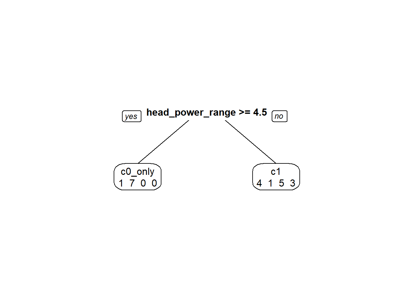
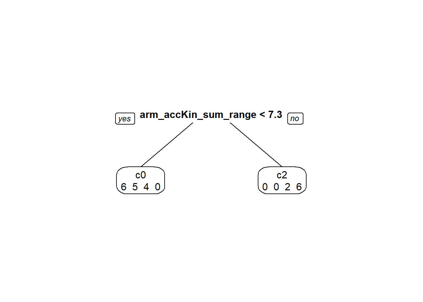
# prepare predictorspredictors <-setdiff(names(data_ges), "correction_info")formula_str <-paste("correction_info ~", paste(predictors, collapse =" + "))# Convert the formula string to a formula objectgesTree_formula <-as.formula(formula_str)# Now use the formula in rpartgesTree <-rpart(formula = gesTree_formula, data = data_ges, method='class', # Specify that it's a classification treecontrol =rpart.control(maxdepth =5) # Control parameters for the 'rpart' function)prp( gesTree, # The decision tree object to be visualizedextra =1, # Show extra information (like node statistics) in the plotvarlen =0, # Length of variable names (0 means auto-determined)faclen =0# Length of factor levels displayed on the plot (increase as needed))
Split the data
# This method should ensure that all levels of our dependent variable are present in both sets# Ensure each level is present in both setstrain_data <- data_ges %>%group_by(correction_info) %>%sample_frac(0.8, replace =FALSE) %>%ungroup()# Assign the remaining samples to the test settest_data <-anti_join(data_ges, train_data)
Building the untuned model.
# Untuned Model with importance (permutation) option setgesUntuned <-ranger(y = train_data$correction_info,x = train_data[,0:324],num.trees =500,importance ="permutation")predictions <-predict(gesUntuned, data = test_data)$predictions# Create a confusion matrixconfusion_matrix <-confusionMatrix(predictions, test_data$correction_info)# Print the confusion matrixprint(confusion_matrix)
Confusion Matrix and Statistics

          Reference
Prediction c0 c0_only c1 c2
   c0       0       2  1  0
   c0_only  1       0  0  0
   c1       0       0  0  1
   c2       0       0  0  0

Overall Statistics

               Accuracy : 0
                 95% CI : (0, 0.5218)
    No Information Rate : 0.4
    P-Value [Acc > NIR] : 1

                  Kappa : -0.3158

 Mcnemar's Test P-Value : NA

Statistics by Class:

                     Class: c0 Class: c0_only Class: c1 Class: c2
Sensitivity              0.000         0.0000     0.000       0.0
Specificity              0.250         0.6667     0.750       1.0
Pos Pred Value           0.000         0.0000     0.000       NaN
Neg Pred Value           0.500         0.5000     0.750       0.8
Prevalence               0.200         0.4000     0.200       0.2
Detection Rate           0.000         0.0000     0.000       0.0
Detection Prevalence     0.600         0.2000     0.200       0.0
Balanced Accuracy        0.125         0.3333     0.375       0.5
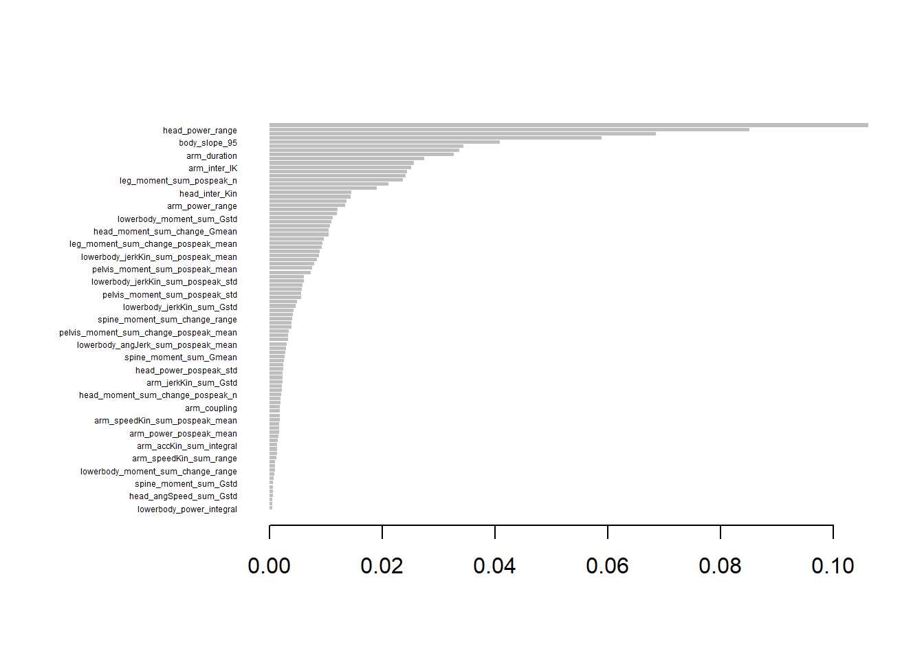
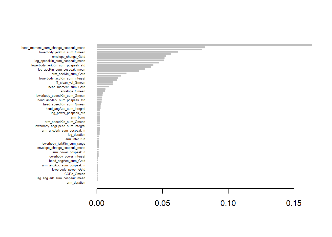
# Calculate feature importancefeature_importance <-importance(gesUntuned, num.threads =1, type =1) # Convert to data framefeature_importance <-as.data.frame(feature_importance, stringsAsFactors =FALSE)feature_importance$Feature <-rownames(feature_importance)colnames(feature_importance) <-c("Importance", "Feature")# Sort by importancesorted_feature_importance <- feature_importance[order(-feature_importance$Importance), ]# Print sorted feature importancehead(sorted_feature_importance, n=10)
# Define the number of CPU cores to usenum_cores <-detectCores()# Create a cluster with specified number of corescl <-makeCluster(num_cores)
Tuning the random forest.
tuneGes <-makeClassifTask(data = data_ges[,0:325],target ="correction_info")tuneGes <-tuneRanger(tuneGes,measure =list(multiclass.brier),num.trees =500)# Return hyperparameter values#tuneGes# Recommended parameter settings: # mtry min.node.size sample.fraction# 1 57 4 0.2279307# Results: # multiclass.brier exec.time# 1 0.790973 0.164gesTuned <-ranger(y = train_data$correction_info,x = train_data[,0:324], num.trees =5000, mtry =57, # Set the recommended mtry value (number of features).min.node.size =4, # Set the recommended min.node.size value (number of samples before a node terminates).sample.fraction =0.2279307, # Set the recommended sample fraction value.(% of data for bagging).importance ="permutation"# Permutation is a computationally intensive test.)predictions <-predict(gesTuned, data = test_data)$predictions# Create a confusion matrixconfusion_matrix <-confusionMatrix(predictions, test_data$correction_info)# Print the confusion matrixprint(confusion_matrix)
Confusion Matrix and Statistics

          Reference
Prediction c0 c0_only c1 c2
   c0       0       0  0  0
   c0_only  1       2  1  1
   c1       0       0  0  0
   c2       0       0  0  0

Overall Statistics

               Accuracy : 0.4
                 95% CI : (0.0527, 0.8534)
    No Information Rate : 0.4
    P-Value [Acc > NIR] : 0.663

                  Kappa : 0

 Mcnemar's Test P-Value : NA

Statistics by Class:

                     Class: c0 Class: c0_only Class: c1 Class: c2
Sensitivity                0.0            1.0       0.0       0.0
Specificity                1.0            0.0       1.0       1.0
Pos Pred Value             NaN            0.4       NaN       NaN
Neg Pred Value             0.8            NaN       0.8       0.8
Prevalence                 0.2            0.4       0.2       0.2
Detection Rate             0.0            0.4       0.0       0.0
Detection Prevalence       0.0            1.0       0.0       0.0
Balanced Accuracy          0.5            0.5       0.5       0.5
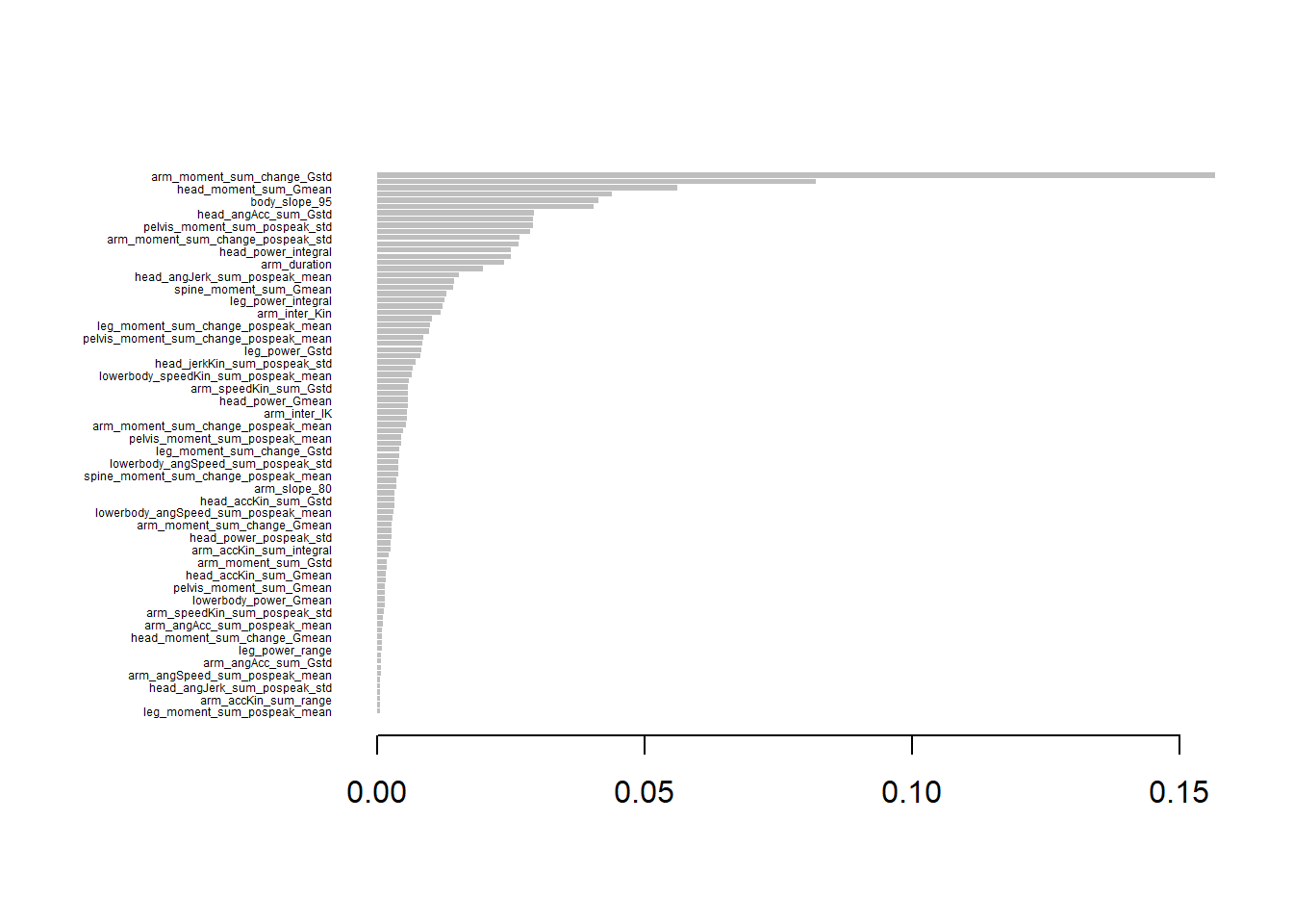
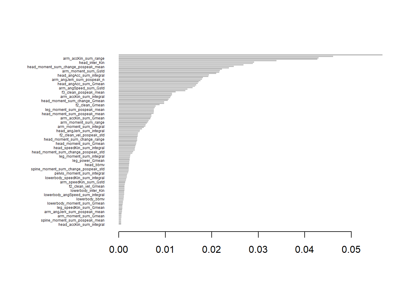
# Calculate feature importancefeature_importance <-importance(gesTuned, num.threads =1, type =1) # Convert to data framefeature_importance <-as.data.frame(feature_importance, stringsAsFactors =FALSE)feature_importance$Feature <-rownames(feature_importance)colnames(feature_importance) <-c("Importance", "Feature")# Sort by importancesorted_feature_importance <- feature_importance[order(-feature_importance$Importance), ]# Print sorted feature importancehead(sorted_feature_importance, n=10)
# Detect the number of available corescores <-detectCores() #- 1 # Leave one core free# Create a cluster with the detected number of corescl <-makeCluster(cores)# Register the parallel backendregisterDoParallel(cl)
Define the grid and estimate runtime.
grid_tune <-expand.grid(nrounds =c(5000, 10000), max_depth =c(3, 6), eta =c(0.05, 0.1), gamma =c(0.1), colsample_bytree =c(0.6, 0.8), min_child_weight =c(1), subsample =c(0.75, 1.0))# Calculate total combinationstotal_combinations <-nrow(grid_tune)# Estimate single model run time (assume 1 minute per run)single_model_time <-10# minute# Total runs for cross-validationfolds <-5total_runs <- total_combinations * folds# Total time estimation without parallel processingtotal_time <- total_runs * single_model_time # in minutes# Convert to hourstotal_time_hours <- total_time /60# Output estimated time without parallel processingprint(paste("Estimated time for grid search without parallel processing:", total_time_hours, "hours"))
[1] "Estimated time for grid search without parallel processing: 26.6666666666667 hours"
# Parallel processing with 4 corescores <-24total_time_parallel <- total_time / cores # in minutes# Convert to hourstotal_time_parallel_hours <- total_time_parallel /60# Output estimated time with parallel processingprint(paste("Estimated time for grid search with", cores, "cores:", total_time_parallel_hours, "hours"))
[1] "Estimated time for grid search with 24 cores: 1.11111111111111 hours"
# Set seed for reproducibilityset.seed(998)# Set up train controltrain_control <-trainControl(method ="cv", # Cross-validationnumber =5, # 5-fold cross-validationallowParallel =TRUE# Enable parallel processing)# Define the number of subsetsnumSubsets <-5# Load data if neededgesDataXGB <-read_csv(paste0(datasets, "gesDataXGB.csv"))# Ensure 'correction_info' is a factorgesDataXGB$correction_info <-as.factor(gesDataXGB$correction_info)# Remove rows with only NA valuesgesDataXGB <- gesDataXGB[rowSums(is.na(gesDataXGB)) <ncol(gesDataXGB), ]# Split data by levels of 'correction_info'correction_levels <-levels(gesDataXGB$correction_info)split_data <-split(gesDataXGB, gesDataXGB$correction_info)# Initialize a list to store subsetsgesSubsets <-vector("list", length = numSubsets)# Distribute rows for each level equally across subsetsfor (level in correction_levels) { level_data <- split_data[[level]] subset_sizes <-rep(floor(nrow(level_data) / numSubsets), numSubsets) remainder <-nrow(level_data) %% numSubsets# Distribute remainder rows randomlyif (remainder >0) { subset_sizes[seq_len(remainder)] <- subset_sizes[seq_len(remainder)] +1 }# Shuffle rows of the level and assign to subsets shuffled_data <- level_data[sample(nrow(level_data)), ] indices <-cumsum(c(0, subset_sizes))for (i in1:numSubsets) {if (is.null(gesSubsets[[i]])) { gesSubsets[[i]] <- shuffled_data[(indices[i] +1):indices[i +1], ] } else { gesSubsets[[i]] <-rbind(gesSubsets[[i]], shuffled_data[(indices[i] +1):indices[i +1], ]) } }}# Naming the subsetsnames(gesSubsets) <-paste0("gesData", 1:numSubsets)# Verify balance in subsetsfor (i in1:numSubsets) {cat("Subset", i, "contains rows:", nrow(gesSubsets[[i]]), "and levels:\n")print(table(gesSubsets[[i]]$correction_info))}
[13:45:07] WARNING: src/learner.cc:553:
  If you are loading a serialized model (like pickle in Python, RDS in R) generated by
  older XGBoost, please export the model by calling `Booster.save_model` from that version
  first, then load it back in current version. See:

    https://xgboost.readthedocs.io/en/latest/tutorials/saving_model.html

  for more details about differences between saving model and serializing.
[13:45:08] WARNING: src/learner.cc:553:
  If you are loading a serialized model (like pickle in Python, RDS in R) generated by
  older XGBoost, please export the model by calling `Booster.save_model` from that version
  first, then load it back in current version. See:

    https://xgboost.readthedocs.io/en/latest/tutorials/saving_model.html

  for more details about differences between saving model and serializing.
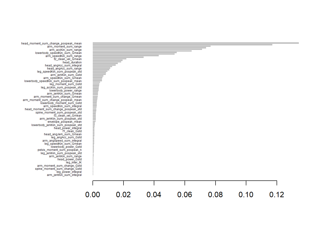
# Compute confusion matricesgesCm1 <-confusionMatrix(gesPredictions1, gesData5$correction_info)gesCm2 <-confusionMatrix(gesPredictions2, gesData4$correction_info)gesCm3 <-confusionMatrix(gesPredictions3, gesData3$correction_info)gesCm4 <-confusionMatrix(gesPredictions4, gesData2$correction_info)gesCm5 <-confusionMatrix(gesPredictions5, gesData1$correction_info)# Extract p-values (you need to define how to extract these based on your metric, here assumed to be some metric from confusion matrix)gesPValues <-c(gesCm1$overall['AccuracyPValue'], gesCm2$overall['AccuracyPValue'], gesCm3$overall['AccuracyPValue'], gesCm4$overall['AccuracyPValue'], gesCm5$overall['AccuracyPValue'])
Now, to select features along different (uncorrelated) dimensions, we want to connect these results with the results of PCA we performed in this script.
Custom function
# Function to select top 3 features per componentselect_top_features <-function(pc_column, xgb_importance, top_n =3) {# Find common features ranked by XGBoost importance common_features <-intersect(pc_column, xgb_importance$Feature) common_features <- xgb_importance %>%filter(Feature %in% common_features) %>%arrange(Rank) %>%pull(Feature)return(head(common_features, top_n))}
First, we collect 10 features per component that have highest combined ranking from PCA and XGBoost. This means that for each feature we sum up the ranking it obtained in cumulative importance (XGBoost) and loading on a principal component (PCA).
# Rank the features based on XGBoost importance (cumulative)gesCumulativeImportance$XGB_Rank <-rank(-gesCumulativeImportance$Cumulative)# Load in PCA for gestureges_pca <-read_csv(paste0(datasets, "PCA_top_contributors_ges.csv"))# For each PC (PC1, PC2, PC3), rank the features based on their loadingscombined_ranks_per_pc <-list()for (pc inc("PC1", "PC2", "PC3")) {# Extract the features and loadings for the current PC pca_pc_loadings <- ges_pca[, c(pc, paste0(pc, "_Loading"))]colnames(pca_pc_loadings) <-c("Feature", "Loading")# Rank the features based on the absolute loading values (higher loadings should get lower rank) pca_pc_loadings$PCA_Rank <-rank(-abs(pca_pc_loadings$Loading))# Merge PCA loadings with XGBoost importance ranks merged_data <-merge(pca_pc_loadings, gesCumulativeImportance[, c("Feature", "XGB_Rank")], by ="Feature")# Calculate combined rank by summing XGBoost rank and PCA rank merged_data$Combined_Rank <- merged_data$XGB_Rank + merged_data$PCA_Rank# Sort by the combined rank (lower rank is better) sorted_data <- merged_data[order(merged_data$Combined_Rank), ]# Select the top n features based on the combined rank for the current PC top_n_features <-10# Adjust the number of top features as needed combined_ranks_per_pc[[pc]] <-head(sorted_data, top_n_features)}# Output the top features per PC based on combined rankinghead(combined_ranks_per_pc, n=10)
For modelling, we want to pick only three features per component. Which would it be in this case?
# Number of top features to displaytop_n_features <-3# Print the top 3 features per componentfor (pc inc("PC1", "PC2", "PC3")) {cat("\nTop 3 Features for", pc, ":\n")# Get the top 3 features based on combined rank for the current PC top_features <-head(combined_ranks_per_pc[[pc]], top_n_features)# Print the resultsprint(top_features[, c("Feature", "XGB_Rank", "PCA_Rank", "Combined_Rank")])}
Top 3 Features for PC1 :
                Feature XGB_Rank PCA_Rank Combined_Rank
28         arm_inter_IK        6       97           103
25             arm_bbmv       99        5           104
68 head_accKin_sum_Gstd       86       18           104

Top 3 Features for PC2 :
                        Feature XGB_Rank PCA_Rank Combined_Rank
113            head_power_range        2       41            43
41  arm_moment_sum_change_range        3       43            46
109         head_power_integral       14       33            47

Top 3 Features for PC3 :
                        Feature XGB_Rank PCA_Rank Combined_Rank
177        lowerbody_power_Gstd       30        7            37
45  arm_moment_sum_pospeak_mean       20       34            54
208  spine_moment_sum_pospeak_n       26       28            54
Vocalization
Now, we just repeat the whole workflow using data for vocalization-only trials.
# Load indata_voc <-read_csv(paste0(datasets, "voc_clean_df.csv"))# Make predictor a factor variabledata_voc$correction_info <-as.factor(data_voc$correction_info)# Displayhead(data_voc, n=10)
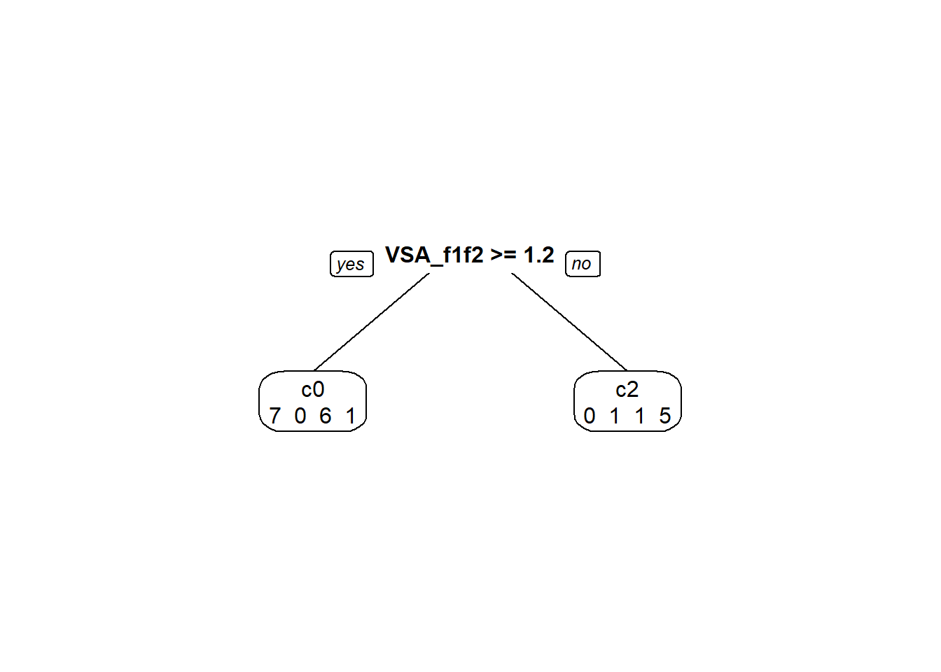
# prepare predictorspredictors <-setdiff(names(data_voc), "correction_info")formula_str <-paste("correction_info ~", paste(predictors, collapse =" + "))# Convert the formula string to a formula objectvocTree_formula <-as.formula(formula_str)# Now use the formula in rpartvocTree <-rpart(formula = vocTree_formula, data = data_voc, method='class', # Specify that it's a classification treecontrol =rpart.control(maxdepth =5) # Control parameters for the 'rpart' function)prp( vocTree, # The decision tree object to be visualizedextra =1, # Show extra information (like node statistics) in the plotvarlen =0, # Length of variable names (0 means auto-determined)faclen =0# Length of factor levels displayed on the plot (increase as needed))
Split the data
Building the untuned model.
# Untuned Model with importance (permutation) option setvocUntuned <-ranger(y = train_data$correction_info,x = train_data[,0:70], # without outcome varnum.trees =500,importance ="permutation")predictions <-predict(vocUntuned, data = test_data)$predictions# Create a confusion matrixconfusion_matrix <-confusionMatrix(predictions, test_data$correction_info)# Print the confusion matrixprint(confusion_matrix)
Confusion Matrix and Statistics

          Reference
Prediction c0 c0_only c1 c2
   c0       0       0  0  1
   c0_only  0       0  0  0
   c1       1       0  1  0
   c2       0       0  0  0

Overall Statistics

               Accuracy : 0.3333
                 95% CI : (0.0084, 0.9057)
    No Information Rate : 0.3333
    P-Value [Acc > NIR] : 0.7037

                  Kappa : 0

 Mcnemar's Test P-Value : NA

Statistics by Class:

                     Class: c0 Class: c0_only Class: c1 Class: c2
Sensitivity             0.0000             NA    1.0000    0.0000
Specificity             0.5000              1    0.5000    1.0000
Pos Pred Value          0.0000             NA    0.5000       NaN
Neg Pred Value          0.5000             NA    1.0000    0.6667
Prevalence              0.3333              0    0.3333    0.3333
Detection Rate          0.0000              0    0.3333    0.0000
Detection Prevalence    0.3333              0    0.6667    0.0000
Balanced Accuracy       0.2500             NA    0.7500    0.5000
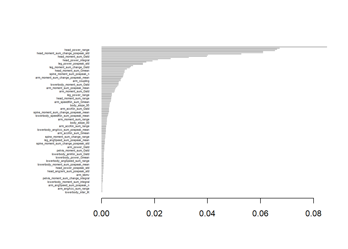
# Calculate feature importancefeature_importance <-importance(vocUntuned, num.threads =1, type =1) # Convert to data framefeature_importance <-as.data.frame(feature_importance, stringsAsFactors =FALSE)feature_importance$Feature <-rownames(feature_importance)colnames(feature_importance) <-c("Importance", "Feature")# Sort by importancesorted_feature_importance <- feature_importance[order(-feature_importance$Importance), ]# Print sorted feature importancehead(sorted_feature_importance, n=10)
# Define the number of CPU cores to usenum_cores <-detectCores()# Create a cluster with specified number of corescl <-makeCluster(num_cores)
Tuning the random forest.
tuneVoc <-makeClassifTask(data = data_voc[,0:71], # with OVtarget ="correction_info")tuneVoc <-tuneRanger(tuneVoc,measure =list(multiclass.brier),num.trees =500)#Return hyperparameter values#tuneVoc# Recommended parameter settings: # mtry min.node.size sample.fraction# 1 6 4 0.522745# Results: # multiclass.brier exec.time# 1 0.7256575 0.166vocTuned <-ranger(y = train_data$correction_info,x = train_data[,0:70], #without OVnum.trees =5000, mtry =6, # Set the recommended mtry value (number of features).min.node.size =4, # Set the recommended min.node.size value (number of samples before a node terminates).sample.fraction =0.522745, # Set the recommended sample fraction value.(% of data for bagging).importance ="permutation"# Permutation is a computationally intensive test.)predictions <-predict(vocTuned, data = test_data)$predictions# Create a confusion matrixconfusion_matrix <-confusionMatrix(predictions, test_data$correction_info)# Print the confusion matrixprint(confusion_matrix)
Confusion Matrix and Statistics

          Reference
Prediction c0 c0_only c1 c2
   c0       0       0  0  1
   c0_only  0       0  0  0
   c1       1       0  1  0
   c2       0       0  0  0

Overall Statistics

               Accuracy : 0.3333
                 95% CI : (0.0084, 0.9057)
    No Information Rate : 0.3333
    P-Value [Acc > NIR] : 0.7037

                  Kappa : 0

 Mcnemar's Test P-Value : NA

Statistics by Class:

                     Class: c0 Class: c0_only Class: c1 Class: c2
Sensitivity             0.0000             NA    1.0000    0.0000
Specificity             0.5000              1    0.5000    1.0000
Pos Pred Value          0.0000             NA    0.5000       NaN
Neg Pred Value          0.5000             NA    1.0000    0.6667
Prevalence              0.3333              0    0.3333    0.3333
Detection Rate          0.0000              0    0.3333    0.0000
Detection Prevalence    0.3333              0    0.6667    0.0000
Balanced Accuracy       0.2500             NA    0.7500    0.5000
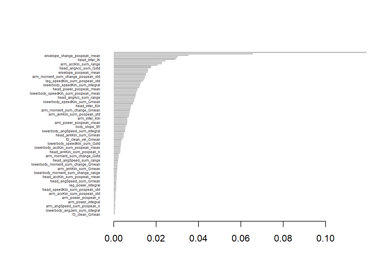
# Calculate feature importancefeature_importance <-importance(vocTuned, num.threads =1, type =1) # Convert to data framefeature_importance <-as.data.frame(feature_importance, stringsAsFactors =FALSE)feature_importance$Feature <-rownames(feature_importance)colnames(feature_importance) <-c("Importance", "Feature")# Sort by importancesorted_feature_importance <- feature_importance[order(-feature_importance$Importance), ]# Print sorted feature importancehead(sorted_feature_importance, n=10)
# Detect the number of available corescores <-detectCores() #- 1 # Leave one core free# Create a cluster with the detected number of corescl <-makeCluster(cores)# Register the parallel backendregisterDoParallel(cl)
Define the grid and estimate runtime.
grid_tune <-expand.grid(nrounds =c(5000, 10000), max_depth =c(3, 6), eta =c(0.05, 0.1), gamma =c(0.1), colsample_bytree =c(0.6, 0.8), min_child_weight =c(1), subsample =c(0.75, 1.0))# Calculate total combinationstotal_combinations <-nrow(grid_tune)# Estimate single model run time (assume 1 minute per run)single_model_time <-10# minute# Total runs for cross-validationfolds <-5total_runs <- total_combinations * folds# Total time estimation without parallel processingtotal_time <- total_runs * single_model_time # in minutes# Convert to hourstotal_time_hours <- total_time /60# Output estimated time without parallel processingprint(paste("Estimated time for grid search without parallel processing:", total_time_hours, "hours"))
[1] "Estimated time for grid search without parallel processing: 26.6666666666667 hours"
# Parallel processing with 4 corescores <-24total_time_parallel <- total_time / cores # in minutes# Convert to hourstotal_time_parallel_hours <- total_time_parallel /60# Output estimated time with parallel processingprint(paste("Estimated time for grid search with", cores, "cores:", total_time_parallel_hours, "hours"))
[1] "Estimated time for grid search with 24 cores: 1.11111111111111 hours"
# Set seed for reproducibilityset.seed(998)# Set up train controltrain_control <-trainControl(method ="cv", # Cross-validationnumber =5, # 5-fold cross-validationallowParallel =TRUE# Enable parallel processing)# Define the number of subsetsnumSubsets <-5# Load MICE-imputed data (using placeholder 'data_ges' as the input dataset)vocDataXGB <-read_csv(paste0(datasets, "vocDataXGB.csv"))# Ensure 'correction_info' is a factorvocDataXGB$correction_info <-as.factor(vocDataXGB$correction_info)# Remove rows with only NA valuesvocDataXGB <- vocDataXGB[rowSums(is.na(vocDataXGB)) <ncol(vocDataXGB), ]# Split data by levels of 'correction_info'correction_levels <-levels(vocDataXGB$correction_info)split_data <-split(vocDataXGB, vocDataXGB$correction_info)# Initialize a list to store subsetsvocSubsets <-vector("list", length = numSubsets)# Distribute rows for each level equally across subsetsfor (level in correction_levels) { level_data <- split_data[[level]] subset_sizes <-rep(floor(nrow(level_data) / numSubsets), numSubsets) remainder <-nrow(level_data) %% numSubsets# Distribute remainder rows randomlyif (remainder >0) { subset_sizes[seq_len(remainder)] <- subset_sizes[seq_len(remainder)] +1 }# Shuffle rows of the level and assign to subsets shuffled_data <- level_data[sample(nrow(level_data)), ] indices <-cumsum(c(0, subset_sizes))for (i in1:numSubsets) {if (is.null(vocSubsets[[i]])) { vocSubsets[[i]] <- shuffled_data[(indices[i] +1):indices[i +1], ] } else { vocSubsets[[i]] <-rbind(vocSubsets[[i]], shuffled_data[(indices[i] +1):indices[i +1], ]) } }}# Naming the subsetsnames(vocSubsets) <-paste0("vocData", 1:numSubsets)# Verify balance in subsetsfor (i in1:numSubsets) {cat("Subset", i, "contains rows:", nrow(vocSubsets[[i]]), "and levels:\n")print(table(vocSubsets[[i]]$correction_info))}
[13:46:05] WARNING: src/learner.cc:553:
  If you are loading a serialized model (like pickle in Python, RDS in R) generated by
  older XGBoost, please export the model by calling `Booster.save_model` from that version
  first, then load it back in current version. See:

    https://xgboost.readthedocs.io/en/latest/tutorials/saving_model.html

  for more details about differences between saving model and serializing.
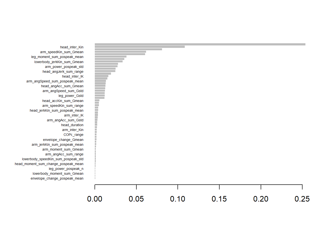
# Compute confusion matricesvocCm1 <-confusionMatrix(vocPredictions1, vocData5$correction_info)vocCm2 <-confusionMatrix(vocPredictions2, vocData4$correction_info)vocCm3 <-confusionMatrix(vocPredictions3, vocData3$correction_info)vocCm4 <-confusionMatrix(vocPredictions4, vocData2$correction_info)vocCm5 <-confusionMatrix(vocPredictions5, vocData1$correction_info)# Extract p-values (you need to define how to extract these based on your metric, here assumed to be some metric from confusion matrix)vocPValues <-c(vocCm1$overall['AccuracyPValue'], vocCm2$overall['AccuracyPValue'], vocCm3$overall['AccuracyPValue'], vocCm4$overall['AccuracyPValue'], vocCm5$overall['AccuracyPValue'])
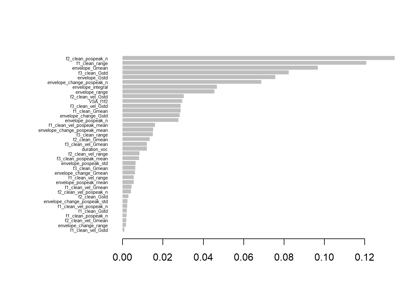
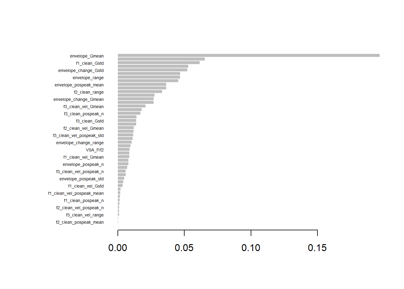
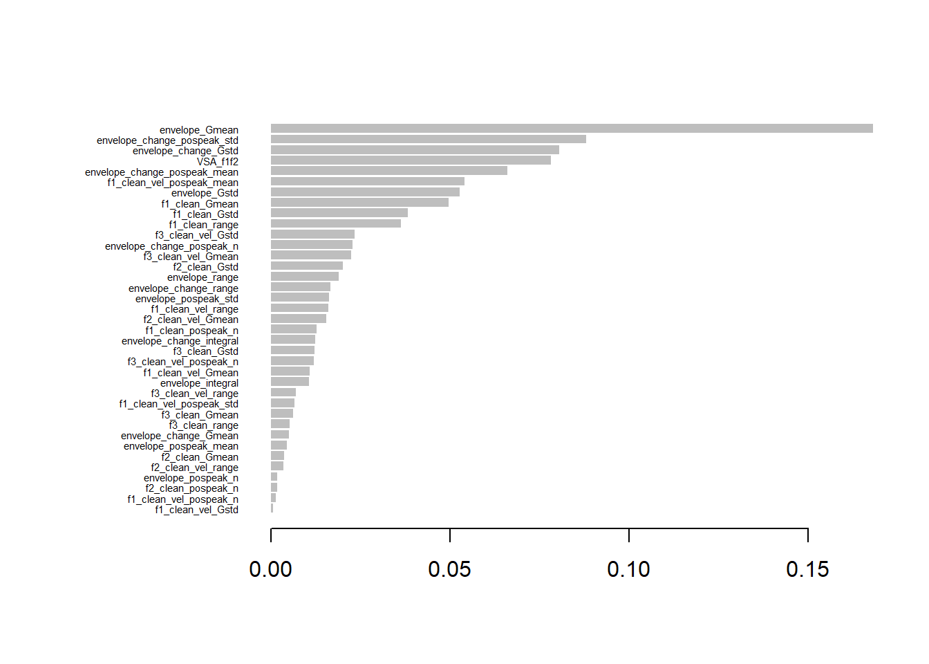
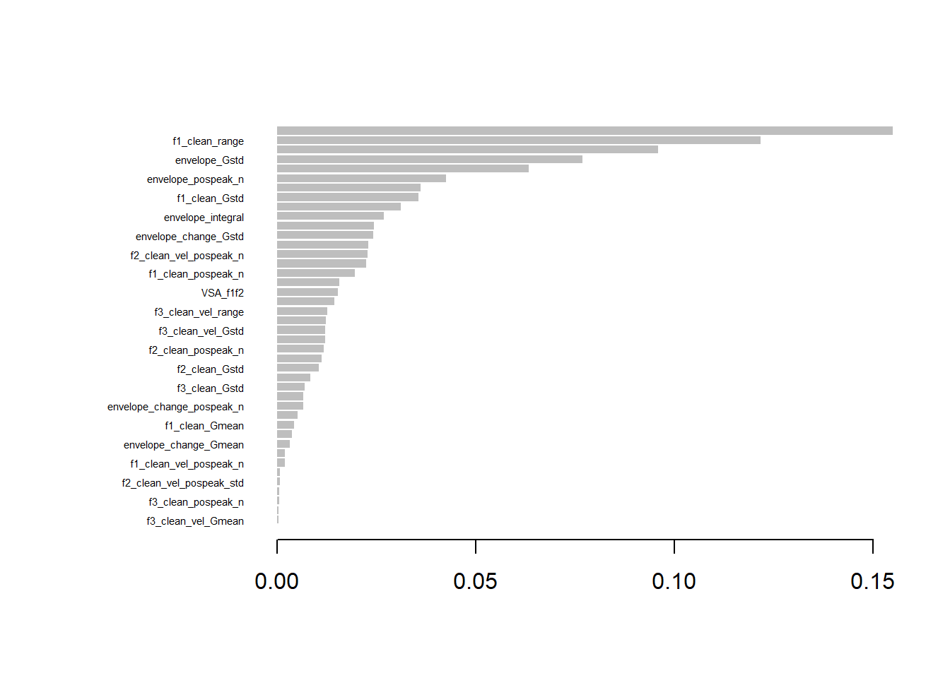
Now let’s collect 10 features per component that have highest combined ranking from PCA and XGBoost. This means that for each feature we sum up the ranking it obtained in cumulative importance (XGBoost) and loading on a principal component (PCA).
# Rank the features based on XGBoost importance (cumulative)vocCumulativeImportance$XGB_Rank <-rank(-vocCumulativeImportance$Cumulative)# Load in PCA for gesturevoc_pca <-read_csv(paste0(datasets, "PCA_top_contributors_voc.csv"))# For each PC (PC1, PC2, PC3), rank the features based on their loadingscombined_ranks_per_pc <-list()for (pc inc("PC1", "PC2", "PC3")) {# Extract the features and loadings for the current PC pca_pc_loadings <- voc_pca[, c(pc, paste0(pc, "_Loading"))]colnames(pca_pc_loadings) <-c("Feature", "Loading")# Rank the features based on the absolute loading values (higher loadings should get lower rank) pca_pc_loadings$PCA_Rank <-rank(-abs(pca_pc_loadings$Loading))# Merge PCA loadings with XGBoost importance ranks merged_data <-merge(pca_pc_loadings, vocCumulativeImportance[, c("Feature", "XGB_Rank")], by ="Feature")# Calculate combined rank by summing XGBoost rank and PCA rank merged_data$Combined_Rank <- merged_data$XGB_Rank + merged_data$PCA_Rank# Sort by the combined rank (lower rank is better) sorted_data <- merged_data[order(merged_data$Combined_Rank), ]# Select the top n features based on the combined rank for the current PC top_n_features <-10# Adjust the number of top features as needed combined_ranks_per_pc[[pc]] <-head(sorted_data, top_n_features)}# Output the top features per PC based on combined rankinghead(combined_ranks_per_pc, n=10)
For modelling, we want to pick three features per component. Which would it be in this case?
# Number of top features to displaytop_n_features <-3# Print the top 3 features per componentfor (pc inc("PC1", "PC2", "PC3")) {cat("\nTop 3 Features for", pc, ":\n")# Get the top 3 features based on combined rank for the current PC top_features <-head(combined_ranks_per_pc[[pc]], top_n_features)# Print the resultsprint(top_features[, c("Feature", "XGB_Rank", "PCA_Rank", "Combined_Rank")])}
Top 3 Features for PC1 :
              Feature XGB_Rank PCA_Rank Combined_Rank
21     f1_clean_range        2        7             9
31 f2_clean_pospeak_n        5        9            14
50           VSA_f1f2        6       10            16

Top 3 Features for PC2 :
             Feature XGB_Rank PCA_Rank Combined_Rank
13 envelope_integral        9        7            16
11    envelope_Gmean        1       20            21
12     envelope_Gstd        3       19            22

Top 3 Features for PC3 :
                Feature XGB_Rank PCA_Rank Combined_Rank
5  envelope_change_Gstd        4       11            15
12        envelope_Gstd        3       12            15
11       envelope_Gmean        1       15            16
Multimodal
Now we take trials from combined modality and follow identical workflow.
# Loaddata_mult <-read_csv(paste0(datasets, "multi_clean_df.csv"))# Make predictor a factor variabledata_mult$correction_info <-as.factor(data_mult$correction_info)# Displayhead(data_mult, n=10)
# prepare predictorspredictors <-setdiff(names(data_mult), "correction_info")formula_str <-paste("correction_info ~", paste(predictors, collapse =" + "))# Convert the formula string to a formula objectmultTree_formula <-as.formula(formula_str)# Now use the formula in rpartmultTree <-rpart(formula = multTree_formula, data = data_mult, method='class', # Specify that it's a classification treecontrol =rpart.control(maxdepth =5) # Control parameters for the 'rpart' function)prp( multTree, # The decision tree object to be visualizedextra =1, # Show extra information (like node statistics) in the plotvarlen =0, # Length of variable names (0 means auto-determined)faclen =0# Length of factor levels displayed on the plot (increase as needed))
Split the data
Building the untuned model.
# Untuned Model with importance (permutation) option setmultUntuned <-ranger(y = train_data$correction_info,x = train_data[,0:394], # without OVnum.trees =500,importance ="permutation")predictions <-predict(multUntuned, data = test_data)$predictions# Create a confusion matrixconfusion_matrix <-confusionMatrix(predictions, test_data$correction_info)# Print the confusion matrixprint(confusion_matrix)
Confusion Matrix and Statistics

          Reference
Prediction c0 c0_only c1 c2
   c0       0       0  0  0
   c0_only  1       0  0  0
   c1       0       1  0  1
   c2       0       0  1  0

Overall Statistics

               Accuracy : 0
                 95% CI : (0, 0.6024)
    No Information Rate : 0.25
    P-Value [Acc > NIR] : 1

                  Kappa : -0.3333

 Mcnemar's Test P-Value : NA

Statistics by Class:

                     Class: c0 Class: c0_only Class: c1 Class: c2
Sensitivity               0.00         0.0000    0.0000    0.0000
Specificity               1.00         0.6667    0.3333    0.6667
Pos Pred Value             NaN         0.0000    0.0000    0.0000
Neg Pred Value            0.75         0.6667    0.5000    0.6667
Prevalence                0.25         0.2500    0.2500    0.2500
Detection Rate            0.00         0.0000    0.0000    0.0000
Detection Prevalence      0.00         0.2500    0.5000    0.2500
Balanced Accuracy         0.50         0.3333    0.1667    0.3333
# Calculate feature importancefeature_importance <-importance(multUntuned, num.threads =1, type =1) # Convert to data framefeature_importance <-as.data.frame(feature_importance, stringsAsFactors =FALSE)feature_importance$Feature <-rownames(feature_importance)colnames(feature_importance) <-c("Importance", "Feature")# Sort by importancesorted_feature_importance <- feature_importance[order(-feature_importance$Importance), ]# Print sorted feature importancehead(sorted_feature_importance, n=10)
# Define the number of CPU cores to usenum_cores <-detectCores()# Create a cluster with specified number of corescl <-makeCluster(num_cores)
Tuning the random forest.
tuneMult <-makeClassifTask(data = data_mult[,0:395], # with OVtarget ="correction_info")tuneMult <-tuneRanger(tuneMult,measure =list(multiclass.brier),num.trees =500)#Return hyperparameter values#tuneMult# Recommended parameter settings: # mtry min.node.size sample.fraction# 1 232 3 0.70919# Results: # multiclass.brier exec.time# 1 0.7385408 0.2multTuned <-ranger(y = train_data$correction_info,x = train_data[,0:394], # without OVnum.trees =5000, mtry =232, # Set the recommended mtry value (number of features).min.node.size =3, # Set the recommended min.node.size value (number of samples before a node terminates).sample.fraction =0.70919, # Set the recommended sample fraction value.(% of data for bagging).importance ="permutation"# Permutation is a computationally intensive test.)predictions <-predict(multTuned, data = test_data)$predictions# Create a confusion matrixconfusion_matrix <-confusionMatrix(predictions, test_data$correction_info)# Print the confusion matrixprint(confusion_matrix)
Confusion Matrix and Statistics

          Reference
Prediction c0 c0_only c1 c2
   c0       0       0  0  0
   c0_only  0       0  0  0
   c1       1       1  0  1
   c2       0       0  1  0

Overall Statistics

               Accuracy : 0
                 95% CI : (0, 0.6024)
    No Information Rate : 0.25
    P-Value [Acc > NIR] : 1

                  Kappa : -0.3333

 Mcnemar's Test P-Value : NA

Statistics by Class:

                     Class: c0 Class: c0_only Class: c1 Class: c2
Sensitivity               0.00           0.00      0.00    0.0000
Specificity               1.00           1.00      0.00    0.6667
Pos Pred Value             NaN            NaN      0.00    0.0000
Neg Pred Value            0.75           0.75      0.00    0.6667
Prevalence                0.25           0.25      0.25    0.2500
Detection Rate            0.00           0.00      0.00    0.0000
Detection Prevalence      0.00           0.00      0.75    0.2500
Balanced Accuracy         0.50           0.50      0.00    0.3333
# Calculate feature importancefeature_importance <-importance(multTuned, num.threads =1, type =1) # Convert to data framefeature_importance <-as.data.frame(feature_importance, stringsAsFactors =FALSE)feature_importance$Feature <-rownames(feature_importance)colnames(feature_importance) <-c("Importance", "Feature")# Sort by importancesorted_feature_importance <- feature_importance[order(-feature_importance$Importance), ]# Print sorted feature importancehead(sorted_feature_importance, n=10)
# Detect the number of available corescores <-detectCores() #- 1 # Leave one core free# Create a cluster with the detected number of corescl <-makeCluster(cores)# Register the parallel backendregisterDoParallel(cl)
Define the grid and estimate runtime.
grid_tune <-expand.grid(nrounds =c(5000, 10000), max_depth =c(3, 6), eta =c(0.05, 0.1), gamma =c(0.1), colsample_bytree =c(0.6, 0.8), min_child_weight =c(1), subsample =c(0.75, 1.0))# Calculate total combinationstotal_combinations <-nrow(grid_tune)# Estimate single model run time (assume 1 minute per run)single_model_time <-10# minute# Total runs for cross-validationfolds <-5total_runs <- total_combinations * folds# Total time estimation without parallel processingtotal_time <- total_runs * single_model_time # in minutes# Convert to hourstotal_time_hours <- total_time /60# Output estimated time without parallel processingprint(paste("Estimated time for grid search without parallel processing:", total_time_hours, "hours"))
[1] "Estimated time for grid search without parallel processing: 26.6666666666667 hours"
# Parallel processing with 4 corescores <-24total_time_parallel <- total_time / cores # in minutes# Convert to hourstotal_time_parallel_hours <- total_time_parallel /60# Output estimated time with parallel processingprint(paste("Estimated time for grid search with", cores, "cores:", total_time_parallel_hours, "hours"))
[1] "Estimated time for grid search with 24 cores: 1.11111111111111 hours"
# Set seed for reproducibilityset.seed(998)# Set up train controltrain_control <-trainControl(method ="cv", # Cross-validationnumber =5, # 5-fold cross-validationallowParallel =TRUE# Enable parallel processing)# Define the number of subsetsnumSubsets <-5# Load MICE-imputed data (using placeholder 'data_ges' as the input dataset)multDataXGB <- data_mult# Ensure 'correction_info' is a factormultDataXGB$correction_info <-as.factor(multDataXGB$correction_info)# Remove rows with only NA valuesmultDataXGB <- multDataXGB[rowSums(is.na(multDataXGB)) <ncol(multDataXGB), ]# Split data by levels of 'correction_info'correction_levels <-levels(multDataXGB$correction_info)split_data <-split(multDataXGB, multDataXGB$correction_info)# Initialize a list to store subsetsmultSubsets <-vector("list", length = numSubsets)# Distribute rows for each level equally across subsetsfor (level in correction_levels) { level_data <- split_data[[level]] subset_sizes <-rep(floor(nrow(level_data) / numSubsets), numSubsets) remainder <-nrow(level_data) %% numSubsets# Distribute remainder rows randomlyif (remainder >0) { subset_sizes[seq_len(remainder)] <- subset_sizes[seq_len(remainder)] +1 }# Shuffle rows of the level and assign to subsets shuffled_data <- level_data[sample(nrow(level_data)), ] indices <-cumsum(c(0, subset_sizes))for (i in1:numSubsets) {if (is.null(multSubsets[[i]])) { multSubsets[[i]] <- shuffled_data[(indices[i] +1):indices[i +1], ] } else { multSubsets[[i]] <-rbind(multSubsets[[i]], shuffled_data[(indices[i] +1):indices[i +1], ]) } }}# Naming the subsetsnames(multSubsets) <-paste0("multData", 1:numSubsets)# Verify balance in subsetsfor (i in1:numSubsets) {cat("Subset", i, "contains rows:", nrow(multSubsets[[i]]), "and levels:\n")print(table(multSubsets[[i]]$correction_info))}
[13:47:05] WARNING: src/learner.cc:553:
  If you are loading a serialized model (like pickle in Python, RDS in R) generated by
  older XGBoost, please export the model by calling `Booster.save_model` from that version
  first, then load it back in current version. See:

    https://xgboost.readthedocs.io/en/latest/tutorials/saving_model.html

  for more details about differences between saving model and serializing.
# Compute confusion matricesmultCm1 <-confusionMatrix(multPredictions1, multData5$correction_info)multCm2 <-confusionMatrix(multPredictions2, multData4$correction_info)multCm3 <-confusionMatrix(multPredictions3, multData3$correction_info)multCm4 <-confusionMatrix(multPredictions4, multData2$correction_info)multCm5 <-confusionMatrix(multPredictions5, multData1$correction_info)# Extract p-values (you need to define how to extract these based on your metric, here assumed to be some metric from confusion matrix)multPValues <-c(multCm1$overall['AccuracyPValue'], multCm2$overall['AccuracyPValue'], multCm3$overall['AccuracyPValue'], multCm4$overall['AccuracyPValue'], multCm5$overall['AccuracyPValue'])
Now let’s collect 10 features per component that have highest combined ranking from PCA and XGBoost. This means that for each feature we sum up the ranking it obtained in cumulative importance (XGBoost) and loading on a principal component (PCA).
# Rank the features based on XGBoost importance (cumulative)multCumulativeImportance$XGB_Rank <-rank(-multCumulativeImportance$Cumulative)# Load in PCA for gesturemult_pca <-read_csv(paste0(datasets, "PCA_top_contributors_multi.csv"))# For each PC (PC1, PC2, PC3), rank the features based on their loadingscombined_ranks_per_pc <-list()for (pc inc("PC1", "PC2", "PC3")) {# Extract the features and loadings for the current PC pca_pc_loadings <- mult_pca[, c(pc, paste0(pc, "_Loading"))]colnames(pca_pc_loadings) <-c("Feature", "Loading")# Rank the features based on the absolute loading values (higher loadings should get lower rank) pca_pc_loadings$PCA_Rank <-rank(-abs(pca_pc_loadings$Loading))# Merge PCA loadings with XGBoost importance ranks merged_data <-merge(pca_pc_loadings, multCumulativeImportance[, c("Feature", "XGB_Rank")], by ="Feature")# Calculate combined rank by summing XGBoost rank and PCA rank merged_data$Combined_Rank <- merged_data$XGB_Rank + merged_data$PCA_Rank# Sort by the combined rank (lower rank is better) sorted_data <- merged_data[order(merged_data$Combined_Rank), ]# Select the top n features based on the combined rank for the current PC top_n_features <-10# Adjust the number of top features as needed combined_ranks_per_pc[[pc]] <-head(sorted_data, top_n_features)}# Output the top features per PC based on combined rankinghead(combined_ranks_per_pc, n=10)
For modelling, we want to pick three features per component. Which would it be in this case?
# Number of top features to displaytop_n_features <-3# Print the top 3 features per componentfor (pc inc("PC1", "PC2", "PC3")) {cat("\nTop 3 Features for", pc, ":\n")# Get the top 3 features based on combined rank for the current PC top_features <-head(combined_ranks_per_pc[[pc]], top_n_features)# Print the resultsprint(top_features[, c("Feature", "XGB_Rank", "PCA_Rank", "Combined_Rank")])}
Top 3 Features for PC1 :
                         Feature XGB_Rank PCA_Rank Combined_Rank
196 lowerbody_speedKin_sum_range       17        1            18
98        head_angJerk_sum_range       14        9            23
94         head_angJerk_sum_Gstd       29       10            39

Top 3 Features for PC2 :
                          Feature XGB_Rank PCA_Rank Combined_Rank
64           envelope_change_Gstd       25     27.0          52.0
157 leg_speedKin_sum_pospeak_mean       19     35.5          54.5
132   leg_accKin_sum_pospeak_mean       24     35.5          59.5

Top 3 Features for PC3 :
                        Feature XGB_Rank PCA_Rank Combined_Rank
47        arm_power_pospeak_std        1       24            25
175 lowerbody_jerkKin_sum_Gmean        6       25            31
104               head_duration        9       28            37
Now we are ready to model the most predictive features to get deeper understanding of their causal relationship with our predictive variable, i.e., communicative attempt.
Chen, Tianqi, and Carlos Guestrin. 2016. “XGBoost: A Scalable Tree Boosting System.” In Proceedings of the 22nd ACM SIGKDD International Conference on Knowledge Discovery and Data Mining, 785–94. KDD ’16. New York, NY, USA: Association for Computing Machinery. https://doi.org/10.1145/2939672.2939785.