def aggregate_keypoints(df, measurement, finalcolname, use):
"""
Aggregates keypoint data by calculating Euclidean sums for predefined groups of keypoints.
Parameters:
-----------
df : pandas.DataFrame
Input dataframe containing keypoint data
measurement : str
Measurement type to filter columns (e.g., 'speed', 'acceleration')
finalcolname : str
Suffix to append to the aggregated column names
use : str
Type of data processing ('kinematics' or 'angles') that determines which keypoint groups to use
Returns:
--------
pandas.DataFrame
DataFrame with additional columns containing aggregated Euclidean sums for each keypoint group
Notes:
------
- For 'kinematics' use, groups keypoints into lower body, legs, head, and arms
- For 'angles' use, groups keypoints into pelvis, spine, lower body, legs, head, and arms
- Each group's Euclidean sum is calculated and stored in a new column with name '{groupname}{finalcolname}'
- The Euclidean sum is calculated as sqrt(sum(values^2)) for each row
"""
if use == 'kinematics':
# group keypoints that belong together
lowerbodycols = ['RHip', 'LHip']
legcols = ['RKnee', 'RAnkle', 'LAnkle', 'LKnee', 'RHeel', 'LHeel']
headcols = ['Head', 'Neck', 'Nose']
armcols = ['RShoulder', 'RElbow', 'RWrist', 'LShoulder', 'LElbow', 'LWrist', 'RIndex', 'LIndex']
groups = [lowerbodycols, legcols, headcols, armcols]
elif use == 'angles':
pelviscols = ['pelvis']
spinecols = ['L5_S1', 'L4_L5', 'L3_L4', 'L2_L3', 'L1_L2', 'L1_T12']
lowerbodycols = ['pelvis', 'hip']
legcols = ['knee', 'ankle', 'subtalar']
headcols = ['neck']
armcols = ['arm', 'elbow', 'wrist', 'pro_sup']
groups = [lowerbodycols, legcols, headcols, armcols, pelviscols, spinecols]
# make subdf only with speed
subdf = df[[x for x in df.columns if measurement in x]]
# loop through each joint group
for group in groups:
# get cols
cols = [x for x in subdf.columns if any(y in x for y in group)]
subdf_temp = subdf[cols]
for index, row in subdf_temp.iterrows():
# get all values of that row
values = row.values
# calculate euclidian sum
euclidian_sum = np.sqrt(np.sum(np.square(values))) ## FLAGGED: possibly normalize
# get a name for new col
if group == lowerbodycols:
colname = 'lowerbody'
elif group == legcols:
colname = 'leg'
elif group == headcols:
colname = 'head'
elif group == armcols:
colname = 'arm'
elif group == pelviscols:
colname = 'pelvis'
elif group == spinecols:
colname = 'spine'
df.loc[index, colname + finalcolname] = euclidian_sum
return df
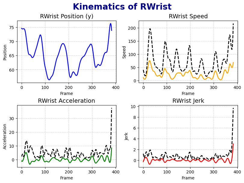
def get_derivatives(df, sr, use):
"""
Computes speed, acceleration, and jerk for each keypoint or angle in the dataframe.
Parameters:
-----------
df : pandas.DataFrame
Input dataframe containing keypoint coordinate data (columns with '_x', '_y', '_z' suffixes)
or angle data (all columns except the first 'time' column)
sr : int or float
Sampling rate in Hz, used to scale finite differences to per-second units
use : str
Type of data processing:
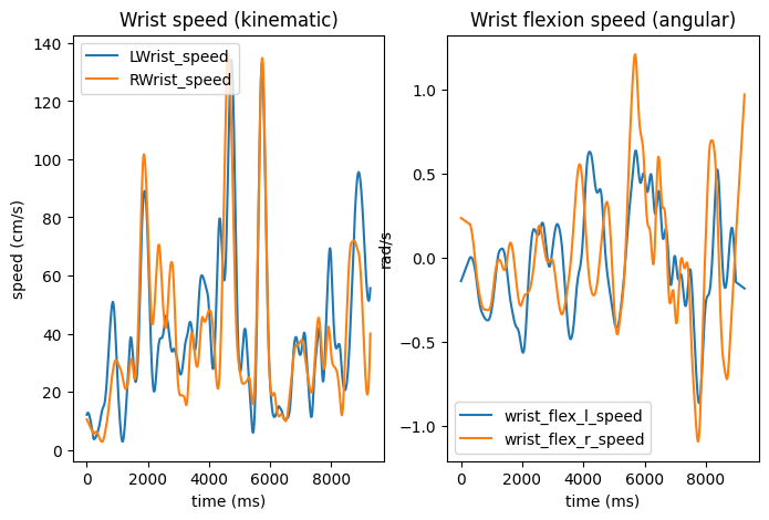
- 'kinematics': computes 3D Euclidean speed, acceleration, and jerk from x/y/z coordinates;
also computes vertical velocity for wrist keypoints
- 'angles': computes angular speed, acceleration, and jerk from angle columns
Returns:
--------
pandas.DataFrame
Input dataframe with additional columns for each keypoint or angle:
'{col}_speed', '{col}_acc', '{col}_jerk'
For wrist keypoints (kinematics only), also adds '{col}_vertvel' (not yet stored in df)
Notes:
------
- Derivatives are computed as finite differences (np.diff) with a leading zero inserted
- Finite differences are scaled by sr to convert from per-sample to per-second units
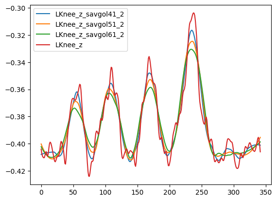
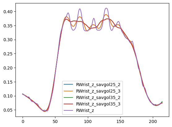
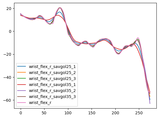
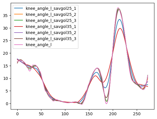
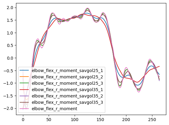
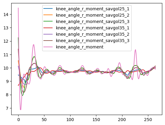
- Each derivative is smoothed with a Savitzky-Golay filter (window=25, order=3 for kinematics;
window=35, order=1 for angles); falls back to (10, 2) then (5, 2) if the signal is too short
- Acceleration is derived from the smoothed speed; jerk from the smoothed acceleration
"""
mtcols = df.columns
if use == 'kinematics':
# get rid of cols that are not x, y or z
mtcols = [x for x in mtcols if '_x' in x or '_y' in x or '_z' in x]
# prepare cols for speed
cols = [x.split('_')[0] for x in mtcols]
colsforspeed = list(set(cols))
# for each unique colname (cols), calculate speed
for col in colsforspeed:
# get x and y columns
x = df[col + '_x']
y = df[col + '_y']
z = df[col + '_z'] # note that y and z are flipped
# calculate speed
speed = np.insert(np.sqrt(np.diff(x)**2 + np.diff(y)**2 + np.diff(z)**2),0,0)
# multiply the values by sr, because now we have values in m/(s/sr)
speed = speed*sr
# smooth
try:
speed = scipy.signal.savgol_filter(speed, 25, 3)
except ValueError:
# if there is a ValueError, it means that the window is too large for the data, so we will use a smaller window
try:
speed = scipy.signal.savgol_filter(speed, 10, 2)
except ValueError:
speed = scipy.signal.savgol_filter(speed, 5, 2)
# if the col contains wrist, we will alco calculate the vertical velocity (z dimension)
if 'Wrist' in col:
verticvel = np.insert(np.diff(z), 0, 0)
verticvel = verticvel*sr
try:
verticvel = scipy.signal.savgol_filter(verticvel, 25, 3)
except ValueError:
# if there is a ValueError, it means that the window is too large for the data, so we will use a smaller window
try:
verticvel = scipy.signal.savgol_filter(verticvel, 10, 2)
except ValueError:
verticvel = scipy.signal.savgol_filter(verticvel, 5, 2)
# derive acceleration
acceleration = np.insert(np.diff(speed), 0, 0)
try:
acceleration = scipy.signal.savgol_filter(acceleration, 25, 3)
except ValueError:
# if there is a ValueError, it means that the window is too large for the data, so we will use a smaller window
try:
acceleration = scipy.signal.savgol_filter(acceleration, 10, 2)
except ValueError:
acceleration = scipy.signal.savgol_filter(acceleration, 5, 2)
# derive jerk
jerk = np.insert(np.diff(acceleration), 0, 0)
try:
jerk = scipy.signal.savgol_filter(jerk, 25, 3)
except ValueError:
# if there is a ValueError, it means that the window is too large for the data, so we will use a smaller window
try:
jerk = scipy.signal.savgol_filter(jerk, 10, 2)
except ValueError:
jerk = scipy.signal.savgol_filter(jerk, 5, 2)
# new_data
new_data = pd.DataFrame({col + '_speed': speed, col + '_acc': acceleration, col + '_jerk': jerk})
df = pd.concat([df, new_data], axis=1)
elif use == 'angles':
# get rid of cols that are not angles (so skip time)
mtcols = mtcols[1:]
# derive speed
for col in mtcols:
speed = np.insert(np.diff(df[col]), 0, 0)
speed = speed*sr
try:
speed = scipy.signal.savgol_filter(speed, 35, 3)
except ValueError:
# if there is a ValueError, it means that the window is too large for the data, so we will use a smaller window
try:
speed = scipy.signal.savgol_filter(speed, 10, 2)
except ValueError:
speed = scipy.signal.savgol_filter(speed, 5, 2)
# derive acceleration
acceleration = np.insert(np.diff(speed), 0, 0)
try:
acceleration = scipy.signal.savgol_filter(acceleration, 35, 3)
except ValueError:
# if there is a ValueError, it means that the window is too large for the data, so we will use a smaller window
try:
acceleration = scipy.signal.savgol_filter(acceleration, 10, 2)
except ValueError:
acceleration = scipy.signal.savgol_filter(acceleration, 5, 2)
# derive jerk
jerk = np.insert(np.diff(acceleration), 0, 0)
try:
jerk = scipy.signal.savgol_filter(jerk, 35, 3)
except ValueError:
# if there is a ValueError, it means that the window is too large for the data, so we will use a smaller window
try:
jerk = scipy.signal.savgol_filter(jerk, 10, 2)
except ValueError:
jerk = scipy.signal.savgol_filter(jerk, 5, 2)
# new_data
new_data = pd.DataFrame({col + '_speed': speed, col + '_acc': acceleration, col + '_jerk': jerk})
df = pd.concat([df, new_data], axis=1)
return df