Computing concept similarity using ConceptNet word embeddings
Overview
Our second hypothesis tests the effect of degree of misunderstanding on the magnitude of effort.
We operationalize degree of misunderstanding as a conceptual similarity between target concept and answer offered by a guesser.
To have a reproducible measure of conceptual similarity, we use the ConceptNet (Speer, Chin, and Havasi 2018) to extract embeddings for concepts used in our study, and calculate cosine similarity between the target concept and guessed answer.
To verify the utility of the cosine similarity, we have collected data from 14 Dutch-native people who were asked to rate the similarity between each pair of words in online anonymous rating study. We then compare the ‘perceived similarity’ with cosine similarity computed from ConceptNet embeddings, to validate the use of ConceptNet embeddings as a measure of conceptual similarity.
Code to load packages and prepare environment
import numpy as npimport osimport globimport pandas as pdimport seaborn as snsimport matplotlib.pyplot as pltimport pingouinimport openpyxlcurfolder = os.getcwd()rawdata = curfolder +'\\..\\00_RAWDATA\\'answerfiles = glob.glob(rawdata +'*\\*.csv', recursive=True)datafolder = curfolder +'\\data\\'# Load all files that have '_1_results' in the name answerfiles_1 = [f for f in answerfiles if'_1_results'in f]# Loop over list and add it into one big dfdf_all1 = pd.DataFrame()forfilein answerfiles_1: df = pd.read_csv(file) df_all1 = pd.concat([df_all1, df], ignore_index=True)df_all1['exp'] =1# Load all files that have '_2_results' in the nameanswerfiles_2 = [f for f in answerfiles if'_2_results'in f]# Loop over list and add it into one big dfdf_all2 = pd.DataFrame()forfilein answerfiles_2: df = pd.read_csv(file) df_all2 = pd.concat([df_all2, df], ignore_index=True)df_all2['exp'] =2# Mergedf_all = pd.concat([df_all1, df_all2], ignore_index=True)# Keep only columns word and answerdf = df_all[['word', 'answer', 'exp']]
First we need to do some data-wrangling to get all in the right format for the embedding extraction and comparison
# Load embeddings from a filedef load_embeddings(file_path): embeddings = {}withopen(file_path, 'r', encoding='utf-8') as f:for line in f: values = line.split() word = values[0] vector = np.array(values[1:], dtype='float32') embeddings[word] = vectorreturn embeddings# Cosine similaritydef cosine_similarity(vec1, vec2): dot_product = np.dot(vec1, vec2) norm_vec1 = np.linalg.norm(vec1) norm_vec2 = np.linalg.norm(vec2)return dot_product / (norm_vec1 * norm_vec2)
We will use multilingual numberbatch to extract words in the original language of experiment - Dutch. While English has better representation in ConceptNet, the English numberbatch does not make distinction between nouns and verbs (so ‘a drink’ and ‘to drink’ have common representation - drink). Because this is important distinction for us, we opt for Dutch embeddings to avoid this problem
Now we take the list of target-answer pairs, transform them into embedding format and perform cosine similarity.
# get the embeddings for the words in the list meanings_enword_embeddings_t = {}for word in meanings_nl: word_embed ='/c/nl/'+ wordif word_embed in embeddings: word_embeddings_t[word] = embeddings[word_embed]# get the embeddings for the words in the list answers_enword_embeddings_ans = {}for word in answers_nl: word_embed ='/c/nl/'+ wordif word_embed in embeddings: word_embeddings_ans[word] = embeddings[word_embed]# calculate the similarity between the first word in the list meanings_en and first word in answers_en, second word in meanings_en and second word in answers_en, etc.cosine_similarities = []for i inrange(len(meanings_nl)): word1 = meanings_nl[i] word2 = answers_nl[i] vec1 = word_embeddings_t.get(word1) vec2 = word_embeddings_ans.get(word2)if vec1 isnotNoneand vec2 isnotNone: cosine_sim = cosine_similarity(vec1, vec2) cosine_similarities.append(cosine_sim)else:# print which concepts could not be foundif vec1 isNone:print(f"Concept not found: {word1}")if vec2 isNone:print(f"Concept not found: {word2}") cosine_similarities.append(None)df['cosine_similarity'] = cosine_similarities# Save itdf.to_csv(datafolder +'conceptnet_clean.csv', index=False)
Concept not found: lawaai maken
Concept not found: lawaai maken
Concept not found: schouderhoogte
Concept not found: openduwen
When running the code, we will see that some target or answered concepts are not represented in numberbatch (e.g., if the answer has more than one word).
Because we verified that cosine similarity and perceived similarity are highly correlated (see below), we will collect the missing data through new online rating study.
Comparing cosine similarity against perceived similarity
To validate the use of ConceptNet embeddings as a measure of conceptual similarity, we compare the cosine similarity computed from ConceptNet embeddings with the ‘perceived similarity’ ratings collected in the online anonymous rating study.
The rating study has been introduced to the participants in a way that closely relates to the experiment. The instructions go as follows:
Below is a list of 171 pairs of words. Your task is to go through them and rate on the scale from 0 to 10 how similar they are/feel for you. You can for example imagine that you are playing a game where you need to explain the first word from the pair (e.g., to dance), and someone answers the second word in the pair. In such a situation, how close is the guesser from the intended word? If they answer ‘to dance’, then the two words are completely identical. But if they answer ‘a car’ it is not similar at all. Rate it according to your intuition, there is no incorrect answer. Note that the survey is completely anonymous and we are not collecting any of your personal data, only the ratings.
This is how the survey results look like:
bloem - feest
dansen - juichen
bitter - lekker
vechten - schieten
ademen - ademen
bijten - zombie
zoemen - bij
fluisteren - zee
walgen - vies
langzaam - lekker
...
zout - mes
zuigen - slurpen
zuigen - drinken
zuigen - drink
dik - eten
dik - heerlijk
dik - lekker
ziek - hoesten
ziek - ziek
huilen - huilen
0
1
3
1
7
10
5
8
1
8
0
...
0
8
6
5
6
5
5
8
10
10
1
3
6
1
6
10
4
8
0
8
1
...
2
8
8
8
7
4
5
7
10
10
2
5
8
5
8
10
7
7
2
8
5
...
2
7
7
7
7
5
6
8
10
10
3
4
6
4
8
10
7
9
7
7
0
...
2
7
7
8
6
2
2
8
10
10
4
6
0
5
6
10
7
8
0
6
0
...
0
7
8
7
4
0
0
8
10
10
5
0
4
2
3
10
6
5
2
8
0
...
0
6
6
4
0
0
0
3
10
10
6
0
1
1
6
10
4
8
0
9
0
...
0
5
6
8
2
0
0
7
10
10
7
1
5
1
2
10
3
6
0
4
0
...
1
6
5
4
6
3
4
6
10
10
8
2
3
3
4
10
0
7
0
8
1
...
0
7
0
2
6
4
2
8
10
10
9
0
2
0
2
10
5
0
0
8
0
...
0
0
3
2
0
0
2
5
10
10
10
3
4
4
7
10
4
6
3
8
3
...
4
7
4
6
6
5
6
7
10
10
11
0
2
0
5
10
8
7
3
9
0
...
0
5
2
2
5
2
1
8
10
10
12
0
0
4
0
10
0
2
0
2
0
...
0
1
1
3
3
5
0
2
10
10
13
0
1
2
1
10
0
0
0
0
1
...
0
2
1
0
0
0
0
0
10
10
14 rows × 166 columns
Now we have to calculate mean rating for each pair
# for each column, calculate the mean and save it to a dfdf_survey_means = pd.DataFrame(df_survey.mean()).reset_index()# separate the index, the first part is English, the second part is the answer_endf_survey_means['word'] = df_survey_means['index'].str.split(' - ').str[0]df_survey_means['answer'] = df_survey_means['index'].str.split(' - ').str[1]# get rid of the index columndf_survey_means = df_survey_means.drop(columns='index')# rename the column 0 to mean_similaritydf_survey_means = df_survey_means.rename(columns={0: 'mean_similarity'})##### some corrections ##### get rid of all invisible spaces in answerdf_survey_means['answer'] = df_survey_means['answer'].str.strip()# where word is vangen and answer vagen, change answer to vangen, and add similarity to 10df_survey_means.loc[(df_survey_means['word'] =='vagen') & (df_survey_means['answer'] =='vangen'), 'word'] ='vangen'df_survey_means.loc[(df_survey_means['word'] =='vangen') & (df_survey_means['answer'] =='vangen'), 'mean_similarity'] =10# where word is lopen and answer skien, change answer to skiëndf_survey_means.loc[(df_survey_means['word'] =='lopen') & (df_survey_means['answer'] =='skien'), 'answer'] ='skiën'# add one missing pair vallen-vallen with mean_similarity 10missing_row = pd.DataFrame({'word': ['vallen'], 'answer': ['vallen'], 'mean_similarity': [10]})df_survey_means = pd.concat([df_survey_means, missing_row], ignore_index=True)# displaydf_survey_means.head(15)
mean_similarity
word
answer
0
1.785714
bloem
feest
1
3.214286
dansen
juichen
2
2.357143
bitter
lekker
3
4.642857
vechten
schieten
4
10.000000
ademen
ademen
5
4.285714
bijten
zombie
6
5.785714
zoemen
bij
7
1.285714
fluisteren
zee
8
6.642857
walgen
vies
9
0.785714
langzaam
lekker
10
10.000000
auto
auto
11
10.000000
eten
eten
12
5.285714
ei
eten
13
1.142857
zwemmen
waaien
14
0.500000
snel
waterslang
Now we can merge it with the cosine similarity dataframe
# load in similaritydf_similarity = pd.read_csv(datafolder +'conceptnet_clean.csv')# merge df_survey_means with df on English and answer_endf_final = pd.merge(df_similarity, df_survey_means, on=['word', 'answer'], how='left')# get rid of English 'to beat'df_final = df_final[df_final['English'] !='beat']# and to weepdf_final = df_final[df_final['English'] !='weep']# save itdf_final.to_csv(datafolder +'/df_final_conceptnet.csv', index=False)# Displaydf_final.head(15)
word
answer
exp
English
answer_en
cosine_similarity
mean_similarity
0
bloem
feest
1
flower
party
0.135571
1.785714
1
dansen
juichen
1
to dance
to cheer
0.177888
3.214286
2
bitter
lekker
1
bitter
tasty
0.257505
2.357143
3
vechten
schieten
1
to fight
to shoot
0.205791
4.642857
4
ademen
ademen
1
to breathe
to breathe
1.000000
10.000000
5
bijten
zombie
1
to bite
zombie
0.068596
4.285714
6
zoemen
bij
1
buzz
bee
0.164508
5.785714
7
fluisteren
zee
1
to whisper
sea
0.072605
1.285714
8
walgen
vies
1
disgusted
dirty
0.353700
6.642857
9
langzaam
lekker
1
slow
tasty
0.077073
0.785714
10
auto
auto
1
car
car
1.000000
10.000000
11
eten
eten
1
to eat
to eat
1.000000
10.000000
12
ei
eten
1
egg
to eat
0.233187
5.285714
13
zwemmen
waaien
1
to swim
to blow
0.065727
1.142857
14
snel
waterslang
1
fast
hose
0.081750
0.500000
Now we can finally run correlation
# get rid of all lines where mean_similarity is 10.0 - otherwise we will drag the correlation updf_corr = df_final[df_final['mean_similarity'] !=10.0]feature1 ="cosine_similarity"feature2 ="mean_similarity"# create a sub-dataframe with the selected features, dropping missing valuessubdf = df_corr[[feature1, feature2]].dropna()# compute the correlation coefficient, with Bayes factorcorr_with_bf = pingouin.pairwise_corr(subdf, columns=['cosine_similarity', 'mean_similarity'], method='pearson', alternative='two-sided')# displayprint(corr_with_bf)
                   X                Y   method alternative    n         r  \
0  cosine_similarity  mean_similarity  pearson   two-sided  122  0.730051

         CI95%         p-unc       BF10  power
0  [0.63, 0.8]  1.430306e-21  3.728e+18    1.0
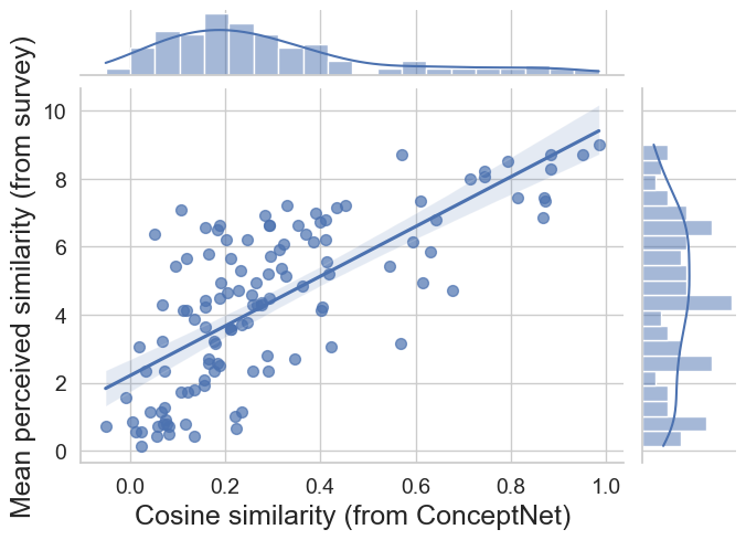
And here we see the relationship visually
The strong correlation (r=0.73) validates the use of ConceptNet embeddings as a measure of conceptual similarity. In the next script, we will load it in together with our effort features.
References
Speer, Robyn, Joshua Chin, and Catherine Havasi. 2018. “ConceptNet 5.5: An Open Multilingual Graph of General Knowledge.” 2018. https://doi.org/10.48550/arXiv.1612.03975.