In this script, we will extract effort-related features from the merged multimodal data we created for each trial in merging script.
Because we are dealing with time-varying data, we will extract number of statistics that characterize both instantaneous as well as cumulative nature of each (acoustic, motion, postural) timeseries in terms of effort.
Before we collect all relevant features, we normalize all time-varying features in the trial by minimum and maximum observed values for that feature for a participant. This is because we want to account for individual differences/strategies in using the whole range of motion and/or acoustic features. We therefore treat effort as a relative measure - but because we cannot access information about the minimum/maximum possible by a participant, we take the maximum and minimum that were observed within the whole experiment.
Code to prepare the environment
# Import packagesimport osimport globimport pandas as pdfrom scipy.signal import find_peaksimport numpy as npimport antropy as entfrom scipy.spatial import ConvexHullimport matplotlib.pyplot as pltfrom mpl_toolkits.mplot3d.art3d import Poly3DCollectionfrom sklearn.decomposition import PCAfrom sklearn.preprocessing import StandardScalerimport umapimport seaborn as snsimport builtinscurfolder = os.getcwd()# Here we store our merged final timeseries datamergedfolder = curfolder +"\\..\\05_finalMerge\\TS_final\\"filestotrack = glob.glob(mergedfolder +"merged_anno*.csv")# Here we store concept similarity dataconceptsimfolder = curfolder +"\\..\\06_ConceptSimilarity\\data\\"# Here we store voice quality measuresvoicefolder = curfolder +"\\..\\03_TS_processing\\TS_acoustics\\"# Here we store other potentially useful datametadatafolder = curfolder +"\\..\\00_RAWDATA\\"# Here we store the final datadatafolder = curfolder +"\\Datasets\\"# These are practice trialspracticetrials = ['0_2_0', '0_2_1', '0_2_19', '0_2_20', '0_2_21', '0_2_22', '0_2_38', '0_2_39', '0_2_40', '0_2_53', '0_2_54', '0_2_55', '0_2_56', '0_2_67', '0_2_68', '0_2_69', '0_2_70', '0_2_71', '0_2_72', '0_2_92', '0_2_93', '0_2_94', '0_2_95', '0_2_96', '0_2_97']# We are interested only in data from part 2, and only those that are not practice trialsfiles_part2 = [] # Collect to list only files that are in part 2 and are not practice trialsforfilein filestotrack: exp_part =file.split("\\")[-1].split("_")[3]if exp_part =="2":ifnotany([x infilefor x in practicetrials]): files_part2.append(file)
Preparing additional metadata
To get additional metadata about the trials, we also need to load in and pre-process some more data, such as:
Similarity between answer and a target concept (computed with ConceptNet). This dataframe has information about the similarity between an answer and performed target concept, computed as cosine similarity of embeddings retrieved from ConceptNet.
Expressibility of a concept. This dataframe has information about expressibility of each concept in a stimuli list. The ratings were acquired from a separate group of people that participated in an online study (Ćwiek et al. n.d.; Kadavá et al. 2024).
Response time. This dataframe has information about how long it took a guesser to provide an answer to a performance, measured from the end of the performance until pressing an Enter to confirm the answer.
This is the similarity dataframe
word
answer
English
answer_en
cosine_similarity
mean_similarity
index
2
vrouw
zwanger
female
pregnant
0.265
4.929
2
3
vrouw
haar
female
hair
0.236
3.714
3
4
vrouw
douchen
female
to shower
0.025
0.571
4
5
verbranden
pijn
to burn
pain
0.119
5.643
5
6
verbranden
verbrand
to burn
burnt
0.883
8.714
6
7
verbranden
heet
to burn
hot
0.412
6.786
7
8
ik
ik
I
I
1.000
10.000
8
9
kauwen
kauwen
to chew
to chew
1.000
10.000
9
10
vliegen
vogel
to fly
bird
0.433
7.143
10
11
vliegen
vliegtuig
to fly
airplane
0.745
8.071
11
12
vliegen
vliegen
to fly
to fly
1.000
10.000
12
13
misschien
denken
maybe
to think
0.567
3.143
13
14
misschien
kiezen
maybe
to choose
0.159
3.643
14
15
misschien
twijfelen
maybe
to doubt
0.284
6.929
15
16
bliksem
graffiti
lightning
graffiti
0.012
0.571
16
This is the expressibility dataframe
word
modality
fit
0
aanraken
gebaren
0.671
1
aanraken
combinatie
0.695
2
aanraken
geluiden
0.207
3
aarde
gebaren
0.539
4
aarde
combinatie
0.524
5
aarde
geluiden
0.195
6
ademen
gebaren
0.782
7
ademen
combinatie
0.808
8
ademen
geluiden
0.785
9
alles
gebaren
0.351
10
alles
combinatie
0.381
11
alles
geluiden
0.118
12
arm (lichaam)
gebaren
0.537
13
arm (lichaam)
combinatie
0.575
14
arm (lichaam)
geluiden
0.127
This is the response time dataframe
TrialID
response_time_sec
2
0_2_2_p0
5.112
3
0_2_3_p0
14.576
4
0_2_4_p0
4.008
5
0_2_5_p0
3.793
6
0_2_6_p0
6.091
7
0_2_7_p0
3.719
8
0_2_8_p0
6.466
9
0_2_9_p0
5.328
10
0_2_10_p0
2.727
11
0_2_11_p0
2.912
12
0_2_12_p0
4.849
13
0_2_13_p0
7.510
14
0_2_14_p0
3.823
15
0_2_15_p0
4.358
16
0_2_16_p0
5.861
Z-scoring to get to relative effort
People can be expected to have a different range of effort, depending on factors including their bodily but also cognitive predispositions. To account for this, we will normalize all data by the means of z-scoring to transform all timeseries such that they represent a deviation from a person’s grand mean for that particulat signal (we will include also data from preceseding experiment that the same participants were performing before this experiment, see preregistration of data collection). We will now collect the means and standard deviations of each timeseries for each participant into a dictionary.
# Loop through all files and get maximum and minimum of all timeserieszscore_dict = {}sessions = ['0']participants = ['p0', 'p1']for session in sessions:forfilein filestotrack: filesession =file.split("\\")[-1].split("_")[2]if filesession == session: filepart =file.split("\\")[-1].split("_")[5].split(".")[0] df_mega_p0 = pd.DataFrame() df_mega_p1 = pd.DataFrame()if filepart =='p0': df_p0 = pd.read_csv(file) df_mega_p0 = pd.concat([df_mega_p0, df_p0])elif filepart =='p1': df_p1 = pd.read_csv(file) df_mega_p1 = pd.concat([df_mega_p1, df_p1]) dfs = [df_mega_p0, df_mega_p1]for df_mega in dfs: numcols = df_mega.select_dtypes(include=[np.number]).columns numcols = [x for x in numcols if'time'notin x]for col in numcols: mean = df_mega[col].mean() std = df_mega[col].std() pcnID = session +"_"+ filepart zscore_dict[pcnID +"_"+ col] = (mean, std)
Now we can check that the normalization of the sample timeseries worked as expected by plotting it against the timeseries before normalization
# Function to z-scoredef zscore(x, col, pcnID, zscore_dict): mean, std = zscore_dict[pcnID +"_"+ col]return (x - mean) / std# Z-score samplesample = files_part2[40]df_sample = pd.read_csv(sample)numcols = df_sample.select_dtypes(include=[np.number]).columns # Normalize only numerical columns (except time)numcols = [x for x in numcols if x !='time']trialID = df_sample['TrialID'].iloc[0]pcnID = trialID.split('_')[0] +'_'+ trialID.split('_')[-1]# Compute all z-scored columns at oncezscore_columns = pd.DataFrame({ col +'_z': df_sample[col].apply(lambda x: zscore(x, col, pcnID, zscore_dict))for col in numcols})# Concatenate the z-scored columns all at once to avoid fragmentationdf_sample = pd.concat([df_sample, zscore_columns], axis=1).copy()# Check the resulting dataframedf_sample.head(15)
time
left_back
right_forward
right_back
left_forward
COPXc
COPYc
COPc
TrialID
FileInfo
...
f1_clean_z
f2_clean_z
f3_clean_z
f1_clean_vel_z
f2_clean_vel_z
f3_clean_vel_z
lowerbody_power_z
leg_power_z
head_power_z
arm_power_z
0
0.0
1.125486
0.804025
1.585540
1.305944
0.000518
0.000133
0.000535
0_2_6_p0
p0_verbranden_combinatie_c1
...
NaN
NaN
NaN
NaN
NaN
NaN
5.454043
0.445892
-0.996332
4.290422
1
2.0
1.125361
0.804328
1.585462
1.305529
0.000438
0.000021
0.000438
0_2_6_p0
p0_verbranden_combinatie_c1
...
NaN
NaN
NaN
NaN
NaN
NaN
5.436372
0.439448
-0.994162
4.274307
2
4.0
1.125285
0.804542
1.585431
1.305204
0.000359
-0.000064
0.000365
0_2_6_p0
p0_verbranden_combinatie_c1
...
NaN
NaN
NaN
NaN
NaN
NaN
5.418702
0.433004
-0.991991
4.258192
3
6.0
1.125250
0.804683
1.585438
1.304959
0.000284
-0.000126
0.000311
0_2_6_p0
p0_verbranden_combinatie_c1
...
NaN
NaN
NaN
NaN
NaN
NaN
5.401031
0.426560
-0.989821
4.242077
4
8.0
1.125250
0.804762
1.585474
1.304782
0.000213
-0.000169
0.000272
0_2_6_p0
p0_verbranden_combinatie_c1
...
NaN
NaN
NaN
NaN
NaN
NaN
5.383361
0.420116
-0.987651
4.225962
5
10.0
1.125279
0.804791
1.585530
1.304662
0.000146
-0.000196
0.000245
0_2_6_p0
p0_verbranden_combinatie_c1
...
NaN
NaN
NaN
NaN
NaN
NaN
5.365690
0.413672
-0.985480
4.209848
6
12.0
1.125331
0.804780
1.585600
1.304591
0.000086
-0.000210
0.000227
0_2_6_p0
p0_verbranden_combinatie_c1
...
NaN
NaN
NaN
NaN
NaN
NaN
5.348020
0.407228
-0.983310
4.193733
7
14.0
1.125401
0.804738
1.585678
1.304559
0.000031
-0.000215
0.000217
0_2_6_p0
p0_verbranden_combinatie_c1
...
NaN
NaN
NaN
NaN
NaN
NaN
5.330349
0.400784
-0.981139
4.177618
8
16.0
1.125485
0.804673
1.585759
1.304560
-0.000018
-0.000212
0.000213
0_2_6_p0
p0_verbranden_combinatie_c1
...
NaN
NaN
NaN
NaN
NaN
NaN
5.312679
0.394340
-0.978969
4.161503
9
18.0
1.125579
0.804591
1.585838
1.304585
-0.000059
-0.000203
0.000212
0_2_6_p0
p0_verbranden_combinatie_c1
...
NaN
NaN
NaN
NaN
NaN
NaN
5.295008
0.387896
-0.976799
4.145389
10
20.0
1.125679
0.804499
1.585913
1.304628
-0.000095
-0.000191
0.000213
0_2_6_p0
p0_verbranden_combinatie_c1
...
NaN
NaN
NaN
NaN
NaN
NaN
5.277338
0.381452
-0.974628
4.129274
11
22.0
1.125781
0.804401
1.585981
1.304683
-0.000123
-0.000177
0.000215
0_2_6_p0
p0_verbranden_combinatie_c1
...
NaN
NaN
NaN
NaN
NaN
NaN
5.259667
0.375008
-0.972458
4.113159
12
24.0
1.125884
0.804302
1.586039
1.304745
-0.000145
-0.000162
0.000217
0_2_6_p0
p0_verbranden_combinatie_c1
...
NaN
NaN
NaN
NaN
NaN
NaN
5.241997
0.368564
-0.970288
4.097044
13
26.0
1.125984
0.804204
1.586087
1.304809
-0.000160
-0.000147
0.000218
0_2_6_p0
p0_verbranden_combinatie_c1
...
NaN
NaN
NaN
NaN
NaN
NaN
5.224326
0.362120
-0.968117
4.080929
14
28.0
1.126080
0.804111
1.586124
1.304872
-0.000169
-0.000134
0.000216
0_2_6_p0
p0_verbranden_combinatie_c1
...
NaN
NaN
NaN
NaN
NaN
NaN
5.206656
0.355676
-0.965947
4.064815
15 rows × 1059 columns
Extracting features: rationale
In the following part, we will be extracting summaries from the existing timeseries that we pre-processed in the previous scripts. The goal is to capture the effort-related features that might be relevant in a repair, i.e., when a participant has to correct themselves to regain understanding with their partner who previously did not understand the performed concept.
Because we are dealing with time-varying data, we will extract number of statistics that characterize both instantaneous as well as cumulative nature of each (acoustic, motion, postural) timeseries in terms of effort. These are:
global mean and standard deviation
number, mean and standard deviation of the peaks (using function find_peaks from scipy.signal). For acceleration and moment change, we also calculate the measurements relating to negative peaks.
range of the values
integral
Additionally, we will compute sample entropy to measure the complexity of a timeseries.
Furthermore, we will utilize measurements that capture characteristics beyond the statistics sketched above. These include:
intermittency (as dimensionless jerk); used in Pouw et al. (2021);
bounding box of movement volume (i.e., gesture space); used in Żywiczyński et al. (2024);
vowel space area (VSA); used in Berisha et al. (2014);
motor complexity; computed as the slope of PCA; similar to Yan et al. (2020);
number of submovements; used in Pouw et al. (2021); Trujillo et al. (2018);
number of moving articulators.
Before proceeding to the feature extraction for all trials, we will first demonstrate the features on a single trial.
This is a dataframe associated with this trial, for now with both zscored and original columns
time
left_back
right_forward
right_back
left_forward
COPXc
COPYc
COPc
TrialID
FileInfo
...
f1_clean_z
f2_clean_z
f3_clean_z
f1_clean_vel_z
f2_clean_vel_z
f3_clean_vel_z
lowerbody_power_z
leg_power_z
head_power_z
arm_power_z
0
0.0
1.125486
0.804025
1.585540
1.305944
0.000518
0.000133
0.000535
0_2_6_p0
p0_verbranden_combinatie_c1
...
NaN
NaN
NaN
NaN
NaN
NaN
5.454043
0.445892
-0.996332
4.290422
1
2.0
1.125361
0.804328
1.585462
1.305529
0.000438
0.000021
0.000438
0_2_6_p0
p0_verbranden_combinatie_c1
...
NaN
NaN
NaN
NaN
NaN
NaN
5.436372
0.439448
-0.994162
4.274307
2
4.0
1.125285
0.804542
1.585431
1.305204
0.000359
-0.000064
0.000365
0_2_6_p0
p0_verbranden_combinatie_c1
...
NaN
NaN
NaN
NaN
NaN
NaN
5.418702
0.433004
-0.991991
4.258192
3
6.0
1.125250
0.804683
1.585438
1.304959
0.000284
-0.000126
0.000311
0_2_6_p0
p0_verbranden_combinatie_c1
...
NaN
NaN
NaN
NaN
NaN
NaN
5.401031
0.426560
-0.989821
4.242077
4
8.0
1.125250
0.804762
1.585474
1.304782
0.000213
-0.000169
0.000272
0_2_6_p0
p0_verbranden_combinatie_c1
...
NaN
NaN
NaN
NaN
NaN
NaN
5.383361
0.420116
-0.987651
4.225962
5
10.0
1.125279
0.804791
1.585530
1.304662
0.000146
-0.000196
0.000245
0_2_6_p0
p0_verbranden_combinatie_c1
...
NaN
NaN
NaN
NaN
NaN
NaN
5.365690
0.413672
-0.985480
4.209848
6
12.0
1.125331
0.804780
1.585600
1.304591
0.000086
-0.000210
0.000227
0_2_6_p0
p0_verbranden_combinatie_c1
...
NaN
NaN
NaN
NaN
NaN
NaN
5.348020
0.407228
-0.983310
4.193733
7
14.0
1.125401
0.804738
1.585678
1.304559
0.000031
-0.000215
0.000217
0_2_6_p0
p0_verbranden_combinatie_c1
...
NaN
NaN
NaN
NaN
NaN
NaN
5.330349
0.400784
-0.981139
4.177618
8
16.0
1.125485
0.804673
1.585759
1.304560
-0.000018
-0.000212
0.000213
0_2_6_p0
p0_verbranden_combinatie_c1
...
NaN
NaN
NaN
NaN
NaN
NaN
5.312679
0.394340
-0.978969
4.161503
9
18.0
1.125579
0.804591
1.585838
1.304585
-0.000059
-0.000203
0.000212
0_2_6_p0
p0_verbranden_combinatie_c1
...
NaN
NaN
NaN
NaN
NaN
NaN
5.295008
0.387896
-0.976799
4.145389
10
20.0
1.125679
0.804499
1.585913
1.304628
-0.000095
-0.000191
0.000213
0_2_6_p0
p0_verbranden_combinatie_c1
...
NaN
NaN
NaN
NaN
NaN
NaN
5.277338
0.381452
-0.974628
4.129274
11
22.0
1.125781
0.804401
1.585981
1.304683
-0.000123
-0.000177
0.000215
0_2_6_p0
p0_verbranden_combinatie_c1
...
NaN
NaN
NaN
NaN
NaN
NaN
5.259667
0.375008
-0.972458
4.113159
12
24.0
1.125884
0.804302
1.586039
1.304745
-0.000145
-0.000162
0.000217
0_2_6_p0
p0_verbranden_combinatie_c1
...
NaN
NaN
NaN
NaN
NaN
NaN
5.241997
0.368564
-0.970288
4.097044
13
26.0
1.125984
0.804204
1.586087
1.304809
-0.000160
-0.000147
0.000218
0_2_6_p0
p0_verbranden_combinatie_c1
...
NaN
NaN
NaN
NaN
NaN
NaN
5.224326
0.362120
-0.968117
4.080929
14
28.0
1.126080
0.804111
1.586124
1.304872
-0.000169
-0.000134
0.000216
0_2_6_p0
p0_verbranden_combinatie_c1
...
NaN
NaN
NaN
NaN
NaN
NaN
5.206656
0.355676
-0.965947
4.064815
15 rows × 1059 columns
Basic statistics
Basic statistics capture properties of the timeseries in several dimensions: - globally (mean, standard deviation of the timeseries, range of the values, rate of the feature) - locally (number, mean and standard deviation of the peaks) - cummulatively (integral of the timeseries)
We also collect the time stamps of the peaks, as we will use them to compute the synchronization between the modalities.
First, to be able to apply the find_peaks function properly, we will need for each column a mean value of the timeseries across all trials. This mean value is then set as the minimum height of a peak for a timeseries
df_list = [] # List to store individual DataFrames before concatenation# First, collect all part2 trials into one z-scoreforfilein files_part2: df = pd.read_csv(file)# Get all numerical cols numcols = df.select_dtypes(include=[np.number]).columns numcols = [x for x in numcols if x !='time'] # Exclude 'time'# Normalize by observed mean and sd for this participant TrialID = df['TrialID'].iloc[0] pcnID = TrialID.split('_')[0] +'_'+ TrialID.split('_')[-1] normalized_cols = { col +'_z': (df[col] - zscore_dict[pcnID +"_"+ col][0]) / zscore_dict[pcnID +"_"+ col][1]for col in numcols } df_normed = pd.DataFrame(normalized_cols)# Add necessary columns df_normed['TrialID'] = df['TrialID'] df_normed['time'] = df['time'] df_list.append(df_normed) # Store in list instead of concatenating immediately# Concatenate all at once to avoid fragmentationdf_mega = pd.concat(df_list, ignore_index=True)# Compute general meansdf_means = {col +'_general_mean': df_mega[col].mean() for col in df_mega.select_dtypes(include=[np.number]).columns if col !='time'}# Compute general stddf_means.update({col +'_general_std': df_mega[col].std() for col in df_mega.select_dtypes(include=[np.number]).columns if col !='time'})df_means = pd.DataFrame([df_means]) # Check the resulting df_meansdf_means.head(15)
left_back_z_general_mean
right_forward_z_general_mean
right_back_z_general_mean
left_forward_z_general_mean
COPXc_z_general_mean
COPYc_z_general_mean
COPc_z_general_mean
audio_z_general_mean
envelope_z_general_mean
envelope_change_z_general_mean
...
f1_clean_z_general_std
f2_clean_z_general_std
f3_clean_z_general_std
f1_clean_vel_z_general_std
f2_clean_vel_z_general_std
f3_clean_vel_z_general_std
lowerbody_power_z_general_std
leg_power_z_general_std
head_power_z_general_std
arm_power_z_general_std
0
-1.8352
1.496059
-1.401405
1.723082
0.039729
0.062733
1.667578
3.723616
0.09084
-0.15375
...
1.596439
1.299107
1.054862
1.94965
1.3957
0.974311
0.857923
1.595838
1.799934
1.763681
1 rows × 1050 columns
Now we can collect basic statistics.
Note that when we look for peaks, we take the mean value for that signal over all trials. Additionally, in timeseries that have both positive and negative values (e.g., acceleration), we will look for both positive and negative peaks.
Custom functions
# Function to calculate stats for a featuredef get_statistics(cols, df, subdf, dictionary, means_df):for col in cols: Gmean = subdf[col].mean() # General mean Gstd = subdf[col].std() # General std# If the col is 2nd derivative of position data, joint kinematics, or moments, we will calculate both positive and negative peaks (by reversing the sign of the data)if'acc'in col or'Acc'in col or'moment_change'in col: ts_mean = means_df[col +'_z_general_mean'].values[0] # get the overall mean of this signal height = ts_mean -2*df_means[col +'_z_general_std'].values[0] # height is mean - 1*std pospeaks, _ = find_peaks(subdf[col], height=height, distance=100) pospeaks_values = subdf.loc[pospeaks, col] pospeaks_times = subdf.loc[pospeaks, "time"].tolist() negpeaks, _ = find_peaks(-subdf[col], height=-height, distance=50, prominence=0.4) negpeaks_values = subdf.loc[negpeaks, col] negpeaks_times = subdf.loc[negpeaks, "time"].tolist() negpeak_mean = negpeaks_values.mean() negpeak_std = negpeaks_values.std() negpeak_n =len(negpeaks_values)else: ts_mean = means_df[col +'_z_general_mean'].values[0] # get the overall mean of this signal height = ts_mean -2*df_means[col +'_z_general_std'].values[0] # height is mean - 1*std pospeaks, _ = find_peaks(subdf[col], height=height, distance=50, prominence=0.4) pospeaks_values = df.loc[pospeaks, col] # Peak values pospeaks_times = df.loc[pospeaks, "time"].tolist() # Peak time# Plot if needed# peak_times = subdf.iloc[pospeaks]['time']# peak_values = subdf.iloc[pospeaks][col]# plt.plot(subdf['time'], subdf[col], label="Signal")# plt.scatter(peak_times, peak_values, color='r', label="Pos Peaks", marker="x")# plt.title(col)# plt.legend()# plt.show() pospeak_mean = pospeaks_values.mean() # Peak mean pospeak_std = pospeaks_values.std() # Peak std pospeak_n =len(pospeaks_values) # Number of peaks negpeak_mean =None negpeak_std =None negpeak_n =None negpeaks_times =None integral = np.trapz(subdf[col]) # Integralrange= subdf[col].max() - subdf[col].min() # Range# Save all in dictionary dictionary[col] = [Gmean, Gstd, pospeak_mean, pospeak_std, pospeak_n, pospeaks_times, negpeak_mean, negpeak_std, negpeak_n, negpeaks_times, integral, range]return dictionary# Function to adapt rowdef adapt_row(row_to_process):for col in row_to_process.columns:# Calculate for all expcet some already calculated measuresif'inter'notin col and'sampEn'notin col and'bbmv'notin col and'duration'notin col: row_to_process[col +'_Gmean'] = row_to_process[col].apply(lambda x: x[0]) row_to_process[col +'_Gstd'] = row_to_process[col].apply(lambda x: x[1]) row_to_process[col +'_pospeak_mean'] = row_to_process[col].apply(lambda x: x[2]) row_to_process[col +'_pospeak_std'] = row_to_process[col].apply(lambda x: x[3]) row_to_process[col +'_pospeak_n'] = row_to_process[col].apply(lambda x: x[4]) row_to_process[col +'_pospeak_times'] = row_to_process[col].apply(lambda x: x[5]) row_to_process[col +'_negpeak_mean'] = row_to_process[col].apply(lambda x: x[6]) row_to_process[col +'_negpeak_std'] = row_to_process[col].apply(lambda x: x[7]) row_to_process[col +'_negpeak_n'] = row_to_process[col].apply(lambda x: x[8]) row_to_process[col +'_negpeak_times'] = row_to_process[col].apply(lambda x: x[9]) row_to_process[col +'_integral'] = row_to_process[col].apply(lambda x: x[10]) row_to_process[col +'_range'] = row_to_process[col].apply(lambda x: x[11])# Now keep only this newly created cols row_final = row_to_process[[col for col in row_to_process.columns ifany(x in col for x in ['Gmean', 'Gstd', 'pospeak_mean', 'pospeak_std', 'pospeak_n', 'sampen', 'inter', 'integral', 'pospeak_times', 'bbmv', 'range', 'duration', 'negpeak_mean', 'negpeak_std', 'negpeak_n', 'negpeak_times'])]]# Get rid of cols with NaNs row_final = row_final.dropna(axis=1, how='all')return row_final
This is a summary of features for this single trial
RWrist_speed_Gmean
RWrist_speed_Gstd
RWrist_speed_pospeak_mean
RWrist_speed_pospeak_std
RWrist_speed_pospeak_n
RWrist_speed_pospeak_times
RWrist_speed_integral
RWrist_speed_range
0
47.434854
34.936351
77.29624
46.952825
9
[316.0, 1100.0, 1732.0, 2232.0, 2850.0, 3216.0...
125349.559904
135.68402
Bounding box of movement volume
Bounding box of movement volume (BBMV) is a measure of the space covered by the participant’s gestures (Żywiczyński et al. 2024). It is computed as the difference between the maximum and minimum values of the timeseries.
Custom functions
# Function to calcuate bounding box of movement volume def get_bbmv(df, group, kp_dict): coordinates = [col for col in df.columns ifany(x in col for x in ['_x', '_y', '_z'])]# Prepare columns that belong to a group (e.g., arm) kp = kp_dict[group] colstoBBMV = [col for col in coordinates ifany(x in col for x in kp)]# Keep only unique names without coordinates kincols =list(set([col.split('_')[0] for col in colstoBBMV])) bbmvs = {}for col in kincols:# Span of x, y, z x_span = df[col +'_x'].max() - df[col +'_x'].min() y_span = df[col +'_y'].max() - df[col +'_y'].min() z_span = df[col +'_z'].max() - df[col +'_z'].min()# Calculate BBMV bbmv = x_span * y_span * z_span bbmvs[col] = bbmv# Get the sum for the whole group bbmv_sum =sum(bbmvs.values())# Natural logarithm bbmv_sum = np.log(bbmv_sum) return bbmv_sum
Using custom function compute_bounding_box, we will compute BBMV for the sample timeseries. (Note that the values are log-transformed.)
BBMV of the current trial: 8.089072657442488
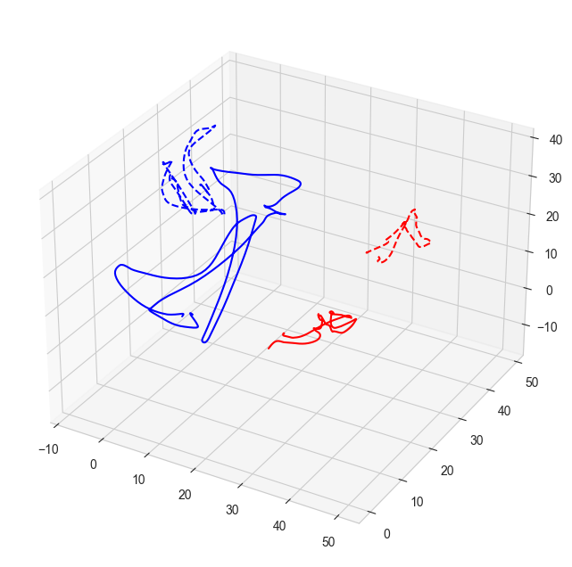
Symmetry of arm movement / multi-movement asymmetry of submovements
Symmetry of arm movement is a measure of how much the participant uses both arms. Symmetrical movement is expected to be less effortful than asymmetrical movement, as asymmetrical movement might require more cognitive resources to coordinate the two arms. We will compute symmetry as the correlation between left and right arm trajectories, similar to Xiong, Quek, and Mcneill (2002). If it’s close to 1, it means that the participant uses both arms in a symmetrical way.
def compute_ArmCoupling(df, keypoints=['Wrist'], dimensions=['x', 'y', 'z'], absolute=True, z=False): correlations = []for kp in keypoints:for dim in dimensions:if z: left_col =f"L{kp}_{dim}_z" right_col =f"R{kp}_{dim}_z"else: left_col =f"L{kp}_{dim}" right_col =f"R{kp}_{dim}"if left_col in df.columns and right_col in df.columns: corr = np.corrcoef(df[left_col], df[right_col])[0, 1] # Pearson correlationif absolute: corr = np.abs(corr) correlations.append(corr)return np.nanmean(correlations) # Average correlation across keypoints and dimensionsdef compute_multimovementAssymetry(df, z=False): joints = ['elbow_flex', 'wrist_flex', 'wrist_dev'] integral_diff_left =0 integral_diff_right =0 joint_integral_differences = []for joint in joints:if z: joint_r_speed =f"{joint}_r_speed_z" joint_l_speed =f"{joint}_l_speed_z"else: joint_r_speed =f"{joint}_r_speed" joint_l_speed =f"{joint}_l_speed"if joint_r_speed in df.columns and joint_l_speed in df.columns:# Compute the integral of velocity (sum of speed over time) for left and right joints integral_velocity_left = np.sum(np.abs(df[joint_l_speed])) # Sum of absolute speed integral_velocity_right = np.sum(np.abs(df[joint_r_speed])) # Sum of absolute speed# Compute the difference in integral of angular velocity between left and right # the more +, the more distance is left is travelling), # but note that because od z-scoring, 0 does not reflect perfect symmetry in distance travelled by both hands joint_integral_diff = integral_velocity_left - integral_velocity_right joint_integral_differences.append(joint_integral_diff)# Accumulate for total integral difference calculation integral_diff_left += integral_velocity_left integral_diff_right += integral_velocity_right# Compute the overall difference in integrated velocities total_integral_difference = np.mean(joint_integral_differences) # Mean of differences across jointsreturn {'mean_integral_difference': total_integral_difference,'joint_integral_differences': joint_integral_differences,'total_left_integral_velocity': integral_diff_left,'total_right_integral_velocity': integral_diff_right }# Example usagecoupling_score = compute_ArmCoupling(df_sample, keypoints=['Wrist', 'Elbow'], dimensions=['x', 'y', 'z'], z=True)arm_asymmetry = compute_multimovementAssymetry(df_sample, z=True)# Plot the trajectoriesplt.figure(figsize=(10, 8))ax = plt.axes(projection='3d')# Plot the left armax.plot3D(df_sample['LWrist_x'], df_sample['LWrist_y'], df_sample['LWrist_z'], 'r')ax.plot3D(df_sample['LElbow_x'], df_sample['LElbow_y'], df_sample['LElbow_z'], 'r', linestyle='--')# Plot the right armax.plot3D(df_sample['RWrist_x'], df_sample['RWrist_y'], df_sample['RWrist_z'], 'b')ax.plot3D(df_sample['RElbow_x'], df_sample['RElbow_y'], df_sample['RElbow_z'], 'b', linestyle='--')plt.show()# Print the symmetry scoreprint("Coupling Score:", coupling_score)print("Arm Asymmetry:", arm_asymmetry['mean_integral_difference'])
Coupling Score: 0.42867744643596634
Arm Asymmetry: -7651.093615100171
Intermittency
Intermittency characterizes the ‘unsmoothess’ of the movement. We follow Pouw et al. (2021)’s adaptation of Hogan and Sternad (2009) and compute dimensionless jerk measure. This measure is computed as the integral of the second derivative of the speed (i.e., jerk) squared multiplied by the duration cubed over the maximum squared velocity.
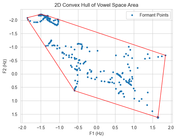
Vowel space area (VSA) is defined as the are of the quadrilateral formed by the four corner vowels /i/, /a/, /u/ and /ɑ/ in the F1-F2 space. It is a measure of the articulatory ‘working’ space and researchers often use it to characterize speech motor control (Berisha et al. 2014).
Despite the fact that we are not dealing with speech data, we can still compute VSA for the first two formants. Following Daniel R. McCloy’s tutorial for R, we will compute VSA for the sample timeseries as the area of the convex hull encompassing all tokens.
# Function to calculate vocal space area (as a convex hull=def getVSA(f1, f2, plot=False):# 2d convex hull points = np.array([f1, f2]).T hull_2d = ConvexHull(points) volume_2d = hull_2d.volume volume_2d = np.log(volume_2d) # natural logif plot: plt.figure() plt.plot(points[:, 0], points[:, 1], 'o', markersize=3, label='Formant Points')for simplex in hull_2d.simplices: plt.plot(points[simplex, 0], points[simplex, 1], 'r-', linewidth=1) plt.xlabel('F1 (Hz)') plt.ylabel('F2 (Hz)') plt.gca().invert_yaxis() plt.legend() plt.title('2D Convex Hull of Vowel Space Area') plt.show()return volume_2d# Calculate on samplef1_clean = df_sample['f1_clean_z'].dropna()f2_clean = df_sample['f2_clean_z'].dropna()vsa = getVSA(f1_clean, f2_clean, plot=True)
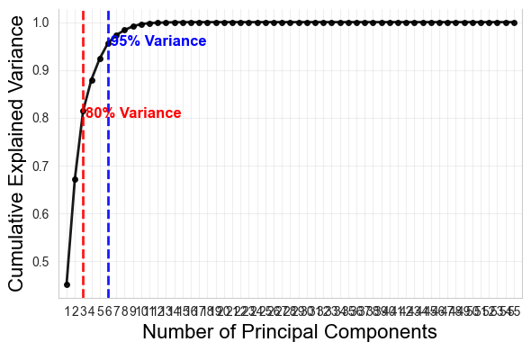
Motor complexity
As a part of exploratory analysis, we also want to assess the motor complexity of the movements as a proxy of coordinative - therefore cognitive - effort relating to the signal.
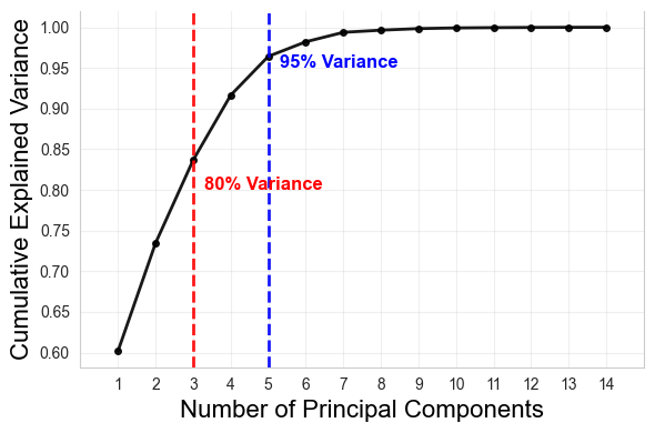
Using OpenSim (Seth et al. 2018), we have been able to extract joint angle measurements for our data. We can use them to assess a motor complexity or alternatively, motor performance of a participant’s movements. We will use Principal Component Analysis (PCA) to assess the motor complexity. We will look at the number of principal components that explain a certain amount of variance in the data and the slope of the explained variance. This will give us a measure of how many (uncorrelated) dimensions/modes cover the most (80 or 95%) of the features of a signal, therefore how complex the movement is in terms of its coordination patterns (Daffertshofer et al. 2004; Yan et al. 2020).
# Function to get the PCAdef get_PCA(df, plot=False):# Step 1: Standardize the Data scaler = StandardScaler() standardized_data = scaler.fit_transform(df)# Step 2: Apply PCA pca = PCA() pca.fit(standardized_data)# Step 3: Explained Variance explained_variance = pca.explained_variance_ratio_ cumulative_explained_variance = explained_variance.cumsum()# Step 4: Find the number of components that explain 95% variance n_components_for_80_variance = np.argmax(cumulative_explained_variance >=0.8) +1# Step 5: Compute the slope for the first n_components_for_95_varianceif n_components_for_80_variance >1: slope_80 = (cumulative_explained_variance[n_components_for_80_variance-1] - cumulative_explained_variance[0]) / (n_components_for_80_variance -1)else: slope_80 = cumulative_explained_variance[0] # Only one component case# 95% variance n_components_for_95_variance = np.argmax(cumulative_explained_variance >=0.95) +1# Step 5: Compute the slope for the first n_components_for_95_varianceif n_components_for_95_variance >1: slope_95 = (cumulative_explained_variance[n_components_for_95_variance-1] - cumulative_explained_variance[0]) / (n_components_for_95_variance -1)else: slope_95 = cumulative_explained_variance[0] # Only one component case# Set Seaborn style for consistency sns.set_style("whitegrid") main_color ="black"# Black for main cumulative variance line red_color ="red"# Basic red for 80% variance threshold blue_color ="blue"# Basic blue for 95% variance thresholdif plot:# get rid of the grid plt.grid(False)# gwt rid of the lines in the backroug plt.gca().spines['top'].set_visible(False)# Adjust x-axis indexing: Components start from 1, not 0 x_values =range(1, len(cumulative_explained_variance) +1)# Plot cumulative explained variance (black line with markers) plt.plot(x_values, cumulative_explained_variance, marker='o', linestyle='-', markersize=4, linewidth=2, color=main_color, alpha=0.9, label='Cumulative Explained Variance')# Add vertical dashed lines for 80% and 95% variance thresholds plt.axvline(x=n_components_for_80_variance, color=red_color, linestyle='--', linewidth=2, alpha=0.9) plt.axvline(x=n_components_for_95_variance, color=blue_color, linestyle='--', linewidth=2, alpha=0.9)# Labels for variance thresholds on the graph plt.text(n_components_for_80_variance +0.3, 0.8, "80% Variance", color=red_color, fontsize=12, fontweight='bold') plt.text(n_components_for_95_variance +0.3, 0.95, "95% Variance", color=blue_color, fontsize=12, fontweight='bold')# Labels and title plt.xlabel('Number of Principal Components', fontsize=16, color='black') plt.ylabel('Cumulative Explained Variance', fontsize=16, color='black')# Ensure x-axis starts at 1 and labels are correctly spaced plt.xticks(x_values) # Explicitly setting x-ticks# Subtle grid plt.grid(True, alpha=0.3) # Make figure smaller plt.gcf().set_size_inches(6, 4)# Tight layout and saving for consistency plt.tight_layout()#xlim plt.xlim(0, len(cumulative_explained_variance) +1) # Adjust x-axis limits plt.show()#plt.close()return n_components_for_80_variance, slope_80, n_components_for_95_variance, slope_95# Calculate on samplePCAcolls_all = ['pelvis_tilt_z', 'pelvis_list_z', 'pelvis_rotation_z', 'pelvis_tx_z','pelvis_ty_z', 'pelvis_tz_z', 'hip_flexion_r_z', 'hip_adduction_r_z','hip_rotation_r_z', 'knee_angle_r_z', 'knee_angle_r_beta_z', 'ankle_angle_r_z','subtalar_angle_r_z', 'hip_flexion_l_z', 'hip_adduction_l_z','hip_rotation_l_z', 'knee_angle_l_z', 'knee_angle_l_beta_z', 'ankle_angle_l_z','subtalar_angle_l_z', 'L5_S1_Flex_Ext_z', 'L5_S1_Lat_Bending_z','L5_S1_axial_rotation_z', 'L4_L5_Flex_Ext_z', 'L4_L5_Lat_Bending_z','L4_L5_axial_rotation_z', 'L3_L4_Flex_Ext_z', 'L3_L4_Lat_Bending_z','L3_L4_axial_rotation_z', 'L2_L3_Flex_Ext_z', 'L2_L3_Lat_Bending_z','L2_L3_axial_rotation_z', 'L1_L2_Flex_Ext_z', 'L1_L2_Lat_Bending_z','L1_L2_axial_rotation_z', 'L1_T12_Flex_Ext_z', 'L1_T12_Lat_Bending_z','L1_T12_axial_rotation_z', 'neck_flexion_z', 'neck_bending_z','neck_rotation_z', 'arm_flex_r_z', 'arm_add_r_z', 'arm_rot_r_z', 'elbow_flex_r_z','pro_sup_r_z', 'wrist_flex_r_z', 'wrist_dev_r_z', 'arm_flex_l_z', 'arm_add_l_z','arm_rot_l_z', 'elbow_flex_l_z', 'pro_sup_l_z', 'wrist_flex_l_z','wrist_dev_l_z']PCAcolls_arm = ['arm_flex_r_z', 'arm_add_r_z', 'arm_rot_r_z', 'elbow_flex_r_z', 'pro_sup_r_z','wrist_flex_r_z', 'wrist_dev_r_z', 'arm_flex_l_z', 'arm_add_l_z', 'arm_rot_l_z','elbow_flex_l_z', 'pro_sup_l_z', 'wrist_flex_l_z', 'wrist_dev_l_z']# Calculate PCA for allsubdf = df_samplePCA_all = get_PCA(subdf[PCAcolls_all], plot=True)print('PCA for whole-body movement complexity', PCA_all)# Calculate PCA for armssubdf = df_samplePCA_arms = get_PCA(subdf[PCAcolls_arm], plot=True)print('PCA for arm movement complexity', PCA_arms)
PCA for whole-body movement complexity (3, 0.18143457258058265, 6, 0.1009103456272205)
PCA for arm movement complexity (3, 0.11732507841208828, 5, 0.09053436514831179)
Extracting features for all trials
Now we will loop through each file (representing a trial), extract the features, add all necessary metadata and save each trial in a overall dataframe. Before any feature is collected, we min-max normalize all data to get to relative feature of effort per participant
import warningswarnings.filterwarnings("ignore")# Initialize the dataframefeatures_df = pd.DataFrame()############################### preparations ################################## These are the names of the columns with movement annotationsmovcols = ['upper_mov', 'arms_mov', 'lower_mov', 'head_mov']# These are our four dimensions for which we have aggregated movement datagroups = ['arm', 'lowerbody', 'leg', 'head']# Mapping between dimension and annotation columnmovcol_keys = {'arm': 'arms_mov', 'lowerbody': 'lower_mov', 'leg': 'lower_mov', 'head': 'head_mov', 'upperbody': 'upper_mov'}# These are groups for BBMVkp_arms = ['RWrist', 'RElbow', 'RShoulder', 'LWrist', 'LElbow', 'LShoulder']kp_lower = ['RAnkle', 'RKnee', 'LAnkle', 'LKnee']kp_legs = ['RAnkle', 'RKnee', 'LAnkle', 'LKnee']kp_head = ['Head']kp_keys = {'arm': kp_arms, 'lowerbody': kp_lower, 'leg': kp_legs, 'head': kp_head}# These are cols associated with balancebalancecols = ['COPc', 'spine_moment_sum', 'pelvis_moment_sum', 'spine_moment_sum_change', 'pelvis_moment_sum_change']# These are cols associated with acousticsvoccols = ['envelope', 'envelope_change', 'f0', 'f1_clean', 'f1_clean_vel', 'f2_clean', 'f2_clean_vel', 'f3_clean', 'f3_clean_vel', 'CoG']PCAcolls_all = ['pelvis_tilt', 'pelvis_list', 'pelvis_rotation', 'pelvis_tx','pelvis_ty', 'pelvis_tz', 'hip_flexion_r', 'hip_adduction_r','hip_rotation_r', 'knee_angle_r', 'knee_angle_r_beta', 'ankle_angle_r','subtalar_angle_r', 'hip_flexion_l', 'hip_adduction_l','hip_rotation_l', 'knee_angle_l', 'knee_angle_l_beta', 'ankle_angle_l','subtalar_angle_l', 'L5_S1_Flex_Ext', 'L5_S1_Lat_Bending','L5_S1_axial_rotation', 'L4_L5_Flex_Ext', 'L4_L5_Lat_Bending','L4_L5_axial_rotation', 'L3_L4_Flex_Ext', 'L3_L4_Lat_Bending','L3_L4_axial_rotation', 'L2_L3_Flex_Ext', 'L2_L3_Lat_Bending','L2_L3_axial_rotation', 'L1_L2_Flex_Ext', 'L1_L2_Lat_Bending','L1_L2_axial_rotation', 'L1_T12_Flex_Ext', 'L1_T12_Lat_Bending','L1_T12_axial_rotation', 'neck_flexion', 'neck_bending','neck_rotation', 'arm_flex_r', 'arm_add_r', 'arm_rot_r', 'elbow_flex_r','pro_sup_r', 'wrist_flex_r', 'wrist_dev_r', 'arm_flex_l', 'arm_add_l','arm_rot_l', 'elbow_flex_l', 'pro_sup_l', 'wrist_flex_l','wrist_dev_l']PCAcolls_arm = ['arm_flex_r', 'arm_add_r', 'arm_rot_r', 'elbow_flex_r', 'pro_sup_r','wrist_flex_r', 'wrist_dev_r', 'arm_flex_l', 'arm_add_l', 'arm_rot_l','elbow_flex_l', 'pro_sup_l', 'wrist_flex_l', 'wrist_dev_l']################################# main loop ##################################forfilein files_part2:print('working on file: ', file) df = pd.read_csv(file)# Get metadata df["concept"] = df["FileInfo"].apply(lambda x: x.split("_")[1]) df["modality"] = df["FileInfo"].apply(lambda x: x.split("_")[2]) df["correction"] = df["FileInfo"].apply(lambda x: x.split("_")[3]) df.drop(columns=["FileInfo"], inplace=True)#################################################### zscoring ##################################################### Get all numerical cols numcols = df.select_dtypes(include=[np.number]).columns numcols = [x for x in numcols if x !='time'] # not time trialID = df['TrialID'][0] pcnID = trialID.split('_')[0] +'_'+ trialID.split('_')[-1] normalized_cols = {}for col in numcols: mean, std = zscore_dict[pcnID +"_"+ col] normalized_cols[col] = df[col].apply(lambda x: (x - mean) / std) df_normed = pd.DataFrame(normalized_cols)# get all cols that are in df but not numcols nonnumcols = [x for x in df.columns if x notin numcols]# add them to the normalized dffor col in nonnumcols: df_normed[col] = df[col]############################### movement feat ################################# Look only into portion of the data where is movement subdf = pd.DataFrame() subdf = df_normed[df_normed["movement_in_trial"] =="movement"] subdf = subdf.reset_index(drop=True)if subdf.shape[0] >0: duration_mov = subdf["time"].iloc[-1] - subdf["time"].iloc[0] # duration submovcols = [col for col in movcols if subdf[col].values[0] =="movement"] numofArt =len(submovcols) # number of articulators# Prepare dictionary to store the values body_sumfeat = {}# Loop over our four dimensions-groups and collect featuresfor group in groups: subsubdf = pd.DataFrame() subsubdf = subdf[subdf[movcol_keys[group]] =="movement"] subsubdf = subsubdf.reset_index(drop=True)# If there is no movement, we set lal values to 0 and continueif subsubdf.shape[0] ==0: body_sumfeat_row = pd.DataFrame() body_sumfeat_row["duration_group"] =0continueelse:# Get the columns that contain group and sum/power (these are cols with aggregated measures) cols = [col for col in subsubdf.columns if group in col and'sum'in col or'power'in col] duration_group = subsubdf["time"].iloc[-1] - subsubdf["time"].iloc[0] # duration# Get statistics body_sumfeat = get_statistics(cols, df_normed, subsubdf, body_sumfeat, df_means) body_sumfeat[group +"_duration"] = duration_group# Calculate intermittency for kinematic measures (from Pose2sim) speed = subsubdf[group +"_speedKin_sum"].values jerk = subsubdf[group +"_jerkKin_sum"].values intermittency = get_intermittency(jerk, speed) intermittency = np.log(intermittency) # natural log body_sumfeat[group +"_inter_Kin"] = intermittency# Calculate intermittency for inverse kinematic measures (from OpenSim) speed = subsubdf[group +"_angSpeed_sum"].values jerk = subsubdf[group +"_angJerk_sum"].values intermittency = get_intermittency(jerk, speed) intermittency = np.log(intermittency) # natural log body_sumfeat[group +"_inter_IK"] = intermittency# Get bounding box of movement volume (BBMV) bbmv_sum = get_bbmv(subsubdf, group, kp_keys) body_sumfeat[group +"_bbmv"] = bbmv_sumelse: duration_mov =0 numofArt =0 body_sumfeat = {}# Convert dictionary to dataframe body_sumfeat_row = pd.DataFrame({key: [value] for key, value in body_sumfeat.items()})# Adapt body_sumfeat_row = adapt_row(body_sumfeat_row)# Add duration and numofArt body_sumfeat_row['duration_mov'] = duration_mov body_sumfeat_row['numofArt'] = numofArt# Get BBMV for the whole body (so concatenate all the groups) bbmv_total = body_sumfeat_row[[col for col in body_sumfeat_row.columns if'bbmv'in col and'rate'notin col]].sum(axis=1) body_sumfeat_row['bbmv_total'] = bbmv_total########################## balance ######################### subdf = pd.DataFrame() subdf = df_normed[df_normed["movement_in_trial"] =="movement"] subdf = subdf.reset_index(drop=True)# Collect features (note that here we collect features for the segment of the general movement, i.e., movement of any body part) balance_sumfeat = {} balance_sumfeat = get_statistics(balancecols, df_normed, subdf, balance_sumfeat, df_means)# Convert dictionary to dataframe balance_sumfeat_row = pd.DataFrame({key: [value] for key, value in balance_sumfeat.items()})# Adapt balance_sumfeat_row = adapt_row(balance_sumfeat_row)######################## acoustics ########################## Check if vocalization existsif"vocalization"notin df_normed.columns:print("No vocalization column in the dataframe") vocfeat_row = pd.DataFrame() # empty rowelse:# Collect features only for the time of vocalizing subdf = pd.DataFrame() subdf = df_normed[df_normed["vocalization"] =="sounding"] subdf = subdf.reset_index(drop=True)if subdf.shape[0] >0: duration_voc = subdf["time"].iloc[-1] - subdf["time"].iloc[0] # duration# Collect features vocfeat_dict = {} vocfeat_dict = get_statistics(voccols, df_normed, subdf, vocfeat_dict, df_means)else:print("No vocalization in the trial") vocfeat_dict = {} duration_voc =0# Convert dictionary to dataframe vocfeat_row = pd.DataFrame({key: [value] for key, value in vocfeat_dict.items()})# Adapt vocfeat_row = adapt_row(vocfeat_row)# Append duration vocfeat_row['duration_voc'] = duration_voc# If f1-f3 are not only nan, calculate the volume of the convex hull (i.e., vowel space area)if subdf['f1_clean'].isnull().all() and subdf['f2_clean'].isnull().all():print("No f1, f2 in the dataframe") vocfeat_row['VSA_f1f2'] =0else: f1_clean = subdf['f1_clean'].dropna() f2_clean = subdf['f2_clean'].dropna() VSA2d = getVSA(f1_clean, f2_clean) # get VSA vocfeat_row['VSA_f1f2'] = VSA2d# Concatenate the rows for movement, balance, and acoustics newrow_concat = pd.concat([body_sumfeat_row, balance_sumfeat_row, vocfeat_row], axis=1)######################################### arms submovements ############################################## Take only the chunk where arms are moving subdf = pd.DataFrame() subdf = df_normed[df_normed["arms_mov"] =="movement"] subdf = subdf.reset_index(drop=True)# Prepare an empty row to store the features newrow_arms = pd.DataFrame()if subdf.shape[0] ==0:print("No movement in arms") arms_submov =0# number of submovements wrists_tempVar =0# temporal variabilityelse:# Count submovements in wrist submovcols = [col for col in subdf.columns if"Wrist"in col and'speed'in col] arms_submov = [] wrists_tempVar = []for col in submovcols:# Calculate the number of peaks that delimit unique submovements ts_mean = df_means[col +'_z_general_mean'].values[0] # get the overall mean of this signal height = ts_mean - df_means[col +'_z_general_std'].values[0] # height is mean - 1*std peaks, _ = find_peaks(subdf[col], height=height, distance=150) arms_submov.append(len(peaks))# Calculate the temporal variability of the submovements peak_times = df_normed.loc[peaks, "time"] intervals = np.diff(peak_times) tempVar = np.std(intervals) wrists_tempVar.append(tempVar)# Append to the row newrow_arms['arms_submovements'] = [arms_submov] newrow_arms['Wrist_tempVar'] = [wrists_tempVar]############################################ arm symmetry ################################################ Calculate symmetry for arms symmetry_score = compute_ArmCoupling(subdf, keypoints=['Wrist', 'Elbow'], dimensions=['x', 'y', 'z']) arm_asymmetry = compute_multimovementAssymetry(subdf) newrow_arms['arm_coupling'] = symmetry_score newrow_arms['arm_asymmetry'] = arm_asymmetry['mean_integral_difference']######################################### Motor complexity (PCA) ######################################### Whole-body complexity subdf = pd.DataFrame() subdf = df_normed.loc[df_normed['movement_in_trial'] =='movement'] subdf = subdf.reset_index(drop=True)if subdf.shape[0] ==0: body_nComp_80 =0 body_slope_80 =0 body_nComp_95 =0 body_slope_95 =0else: bodydf = subdf.loc[:, PCAcolls_all] body_nComp_80, body_slope_80, body_nComp_95, body_slope_95 = get_PCA(bodydf)# Append to the row newrow_concat['body_nComp_80'] = body_nComp_80 newrow_concat['body_slope_80'] = body_slope_80 newrow_concat['body_nComp_95'] = body_nComp_95 newrow_concat['body_slope_95'] = body_slope_95# Arm complexity# Empty subdf subdf = pd.DataFrame() subdf = df_normed.loc[df_normed['arms_mov'] =='movement']if subdf.shape[0] ==0: arm_nComp_80 =0 arm_slope_80 =0 arm_nComp_95 =0 arm_slope_95 =0else: armdf = subdf.loc[:, PCAcolls_arm] arm_nComp_80, arm_slope_80, arm_nComp_95, arm_slope_95 = get_PCA(armdf)# Append to the row newrow_concat['arm_nComp_80'] = arm_nComp_80 newrow_concat['arm_slope_80'] = arm_slope_80 newrow_concat['arm_nComp_95'] = arm_nComp_95 newrow_concat['arm_slope_95'] = arm_slope_95# Concatenate newrow and newrow_arms newrow_final = pd.concat([newrow_concat, newrow_arms], axis=1)# Add metadata newrow_final["TrialID"] = df_normed["TrialID"].values[0] newrow_final["concept"] = df_normed["concept"].values[0] newrow_final["modality"] = df_normed["modality"].values[0] newrow_final["correction"] = df_normed["correction"].values[0]# Add the row the the overal df features_df = pd.concat([features_df, newrow_final], ignore_index=True)############################################## Answer info ############################################## index =int(df_normed["TrialID"].values[0].split("_")[2]) concept = df_normed["concept"].values[0]# Check what was the answer and cosine similarity for the index answer_fol = similaritydata[similaritydata["index"] == index]["answer"].values[0] answer_fol_sim = similaritydata[similaritydata["index"] == index]["cosine_similarity"].values[0]# Check what was the answer and cosine similarity for index before - but only if the previous index has the same concept as the current oneif index -1in similaritydata["index"].values and similaritydata[similaritydata["index"] == index -1]["word"].values[0] == concept: answer_prev = similaritydata[similaritydata["index"] == index -1]["answer"].values[0] answer_prev_sim = similaritydata[similaritydata["index"] == index -1]["cosine_similarity"].values[0]else:#print("previous index doesn't have the same concept") answer_prev =None answer_prev_sim =None# Append to the features_df features_df.loc[features_df["TrialID"] == df_normed["TrialID"].values[0], "answer_fol"] = answer_fol features_df.loc[features_df["TrialID"] == df_normed["TrialID"].values[0], "answer_fol_dist"] = answer_fol_sim features_df.loc[features_df["TrialID"] == df_normed["TrialID"].values[0], "answer_prev"] = answer_prev features_df.loc[features_df["TrialID"] == df_normed["TrialID"].values[0], "answer_prev_dist"] = answer_prev_sim# Check what is the expressibility for the concept & modality express = express_df[(express_df["word"] == concept) & (express_df["modality"] == df_normed["modality"].values[0])]["fit"].values[0] features_df.loc[features_df["TrialID"] == df_normed["TrialID"].values[0], "expressibility"] = express# Add response time from answerdata response_time = answerdata[answerdata["TrialID"] == df_normed["TrialID"].values[0]]["response_time_sec"].values[0] features_df.loc[features_df["TrialID"] == df_normed["TrialID"].values[0], "response_time_sec"] = response_time# Create a concept id to group together corrections of one conceptfor row in features_df.iterrows(): row = row[1] features_df.loc[row.name, "concept_id"] = row["concept"] +"_"+ row["modality"] +"_"+ row["TrialID"].split("_")[-1]# Get rid of columns that have only NA valuesfeatures_df = features_df.dropna(axis=1, how='all')# Round all num cols to 3numcols = features_df.select_dtypes(include=[np.number]).columnsfeatures_df[numcols] = features_df[numcols].round(3)
This is how the dataframe looks like:
arm_duration
arm_inter_Kin
arm_inter_IK
arm_bbmv
lowerbody_duration
lowerbody_inter_Kin
lowerbody_inter_IK
lowerbody_bbmv
leg_duration
leg_inter_Kin
...
f2_clean_pospeak_std
f1_clean_pospeak_std
f1_clean_vel_pospeak_std
CoG_Gmean
CoG_Gstd
CoG_pospeak_mean
CoG_pospeak_std
CoG_integral
CoG_range
concept_id
0
3988.0
26.197
26.728
8.472
2020.0
26.580
26.181
5.400
2020.0
26.759
...
NaN
NaN
NaN
NaN
NaN
NaN
NaN
NaN
NaN
groot_combinatie_p1
1
3868.0
26.674
28.122
8.148
2870.0
28.319
28.291
6.487
2870.0
27.096
...
NaN
NaN
NaN
NaN
NaN
NaN
NaN
NaN
NaN
groot_combinatie_p1
2
4014.0
26.449
27.565
8.465
874.0
23.434
23.040
2.861
874.0
22.945
...
NaN
NaN
NaN
NaN
NaN
NaN
NaN
NaN
NaN
groot_combinatie_p1
3
4046.0
26.207
28.558
8.482
3750.0
28.421
28.796
6.124
3750.0
27.973
...
NaN
NaN
NaN
NaN
NaN
NaN
NaN
NaN
NaN
hoog_combinatie_p1
4
4708.0
26.502
28.717
8.309
4508.0
29.760
28.762
6.005
4508.0
28.679
...
NaN
NaN
NaN
NaN
NaN
NaN
NaN
NaN
NaN
hoog_combinatie_p1
5
4004.0
26.978
28.554
8.699
3598.0
28.801
28.616
5.723
3598.0
28.179
...
NaN
NaN
NaN
NaN
NaN
NaN
NaN
NaN
NaN
hoog_combinatie_p1
6
NaN
NaN
NaN
NaN
784.0
23.222
22.753
2.313
784.0
22.135
...
0.867
NaN
NaN
NaN
NaN
NaN
NaN
NaN
NaN
blij_combinatie_p1
7
5248.0
28.973
31.658
10.919
4930.0
28.905
29.800
14.893
4930.0
28.250
...
NaN
NaN
NaN
NaN
NaN
NaN
NaN
NaN
NaN
vrouw_combinatie_p0
8
1784.0
25.011
24.190
6.604
NaN
NaN
NaN
NaN
NaN
NaN
...
NaN
NaN
NaN
NaN
NaN
NaN
NaN
NaN
NaN
blij_combinatie_p1
9
1284.0
24.278
24.516
5.054
1334.0
25.381
25.483
4.317
1334.0
24.478
...
NaN
NaN
NaN
NaN
NaN
NaN
NaN
NaN
NaN
blij_combinatie_p1
10
1494.0
24.248
24.502
6.483
2944.0
29.247
28.630
5.378
2944.0
26.524
...
NaN
0.018
0.812
NaN
NaN
NaN
NaN
NaN
NaN
vis_combinatie_p1
11
2486.0
25.718
26.035
6.420
780.0
25.181
21.982
2.271
780.0
22.482
...
NaN
NaN
NaN
NaN
NaN
NaN
NaN
NaN
NaN
ruiken_combinatie_p1
12
2968.0
25.494
28.758
8.040
2750.0
28.377
27.107
4.885
2750.0
26.672
...
0.618
NaN
0.552
NaN
NaN
NaN
NaN
NaN
NaN
wind_combinatie_p1
13
3850.0
27.666
27.348
7.419
3366.0
28.208
28.519
5.033
3366.0
28.230
...
0.223
NaN
0.502
NaN
NaN
NaN
NaN
NaN
NaN
heet_combinatie_p1
14
3236.0
26.551
27.446
6.411
NaN
NaN
NaN
NaN
NaN
NaN
...
0.197
0.429
0.347
NaN
NaN
NaN
NaN
NaN
NaN
heet_combinatie_p1
15
5572.0
28.818
28.100
9.814
5158.0
29.833
29.109
6.470
5158.0
29.409
...
NaN
NaN
NaN
NaN
NaN
NaN
NaN
NaN
NaN
heet_combinatie_p1
16
1144.0
23.839
26.291
8.156
324.0
19.470
20.447
0.414
324.0
19.033
...
NaN
NaN
NaN
NaN
NaN
NaN
NaN
NaN
NaN
vrouw_combinatie_p0
17
3816.0
28.001
29.471
10.348
3244.0
27.815
30.057
9.607
3244.0
27.788
...
NaN
NaN
NaN
NaN
NaN
NaN
NaN
NaN
NaN
vogel_gebaren_p0
18
5280.0
28.098
30.942
13.350
5862.0
28.648
31.235
17.882
5862.0
29.740
...
NaN
NaN
NaN
NaN
NaN
NaN
NaN
NaN
NaN
kruipen_gebaren_p0
19
4302.0
28.401
31.164
10.572
4206.0
28.373
31.096
8.402
4206.0
27.451
...
NaN
NaN
NaN
NaN
NaN
NaN
NaN
NaN
NaN
water_gebaren_p0
20
4474.0
27.316
30.376
10.229
4398.0
28.390
32.196
9.064
4398.0
27.665
...
NaN
NaN
NaN
NaN
NaN
NaN
NaN
NaN
NaN
water_gebaren_p0
21
4388.0
27.872
31.225
9.748
3782.0
27.458
30.479
8.428
3782.0
27.529
...
NaN
NaN
NaN
NaN
NaN
NaN
NaN
NaN
NaN
water_gebaren_p0
22
5852.0
29.417
32.048
10.675
5404.0
29.153
30.545
10.334
5404.0
29.056
...
NaN
NaN
NaN
-0.784
1.429
-3.658
0.171
-210.357
5.017
vuur_gebaren_p0
23
2736.0
26.324
27.656
6.547
NaN
NaN
NaN
NaN
NaN
NaN
...
NaN
NaN
NaN
NaN
NaN
NaN
NaN
NaN
NaN
goed_gebaren_p0
24
4256.0
28.675
29.776
8.148
NaN
NaN
NaN
NaN
NaN
NaN
...
NaN
NaN
NaN
NaN
NaN
NaN
NaN
NaN
NaN
goed_gebaren_p0
25
2516.0
26.234
27.815
7.774
884.0
23.300
25.890
6.598
884.0
23.423
...
NaN
NaN
NaN
NaN
NaN
NaN
NaN
NaN
NaN
horen_gebaren_p0
26
5832.0
29.027
31.043
11.094
3936.0
27.904
29.471
11.080
3936.0
27.885
...
NaN
NaN
NaN
NaN
NaN
NaN
NaN
NaN
NaN
vrouw_combinatie_p0
27
4504.0
28.604
30.892
9.939
4266.0
27.764
29.475
11.045
4266.0
28.404
...
NaN
NaN
NaN
NaN
NaN
NaN
NaN
NaN
NaN
ver_gebaren_p0
28
5946.0
28.473
30.925
9.779
5136.0
28.712
30.358
9.084
5136.0
28.117
...
NaN
NaN
NaN
NaN
NaN
NaN
NaN
NaN
NaN
ver_gebaren_p0
29
6100.0
29.300
31.243
10.521
6030.0
29.592
30.960
9.672
6030.0
30.037
...
NaN
NaN
NaN
NaN
NaN
NaN
NaN
NaN
NaN
ver_gebaren_p0
30
3004.0
26.079
26.368
7.253
2686.0
28.219
27.971
4.870
2686.0
27.750
...
NaN
NaN
NaN
NaN
NaN
NaN
NaN
NaN
NaN
blazen_gebaren_p1
31
3918.0
28.358
28.936
8.394
3366.0
28.669
28.833
5.086
3366.0
28.617
...
NaN
NaN
NaN
NaN
NaN
NaN
NaN
NaN
NaN
geven_gebaren_p1
32
3918.0
28.120
29.766
9.343
1692.0
26.370
26.244
4.733
1692.0
24.816
...
NaN
NaN
NaN
NaN
NaN
NaN
NaN
NaN
NaN
geven_gebaren_p1
33
1202.0
23.839
27.274
8.980
1590.0
25.566
27.624
11.326
1590.0
25.540
...
NaN
NaN
NaN
NaN
NaN
NaN
NaN
NaN
NaN
verbranden_combinatie_p0
34
2352.0
25.612
25.352
6.061
NaN
NaN
NaN
NaN
NaN
NaN
...
NaN
NaN
NaN
NaN
NaN
NaN
NaN
NaN
NaN
kat_gebaren_p1
35
1954.0
25.071
25.036
6.560
1992.0
27.080
26.978
4.535
1992.0
25.756
...
NaN
NaN
NaN
NaN
NaN
NaN
NaN
NaN
NaN
lachen_gebaren_p1
36
4400.0
27.535
28.492
5.513
NaN
NaN
NaN
NaN
NaN
NaN
...
NaN
NaN
NaN
NaN
NaN
NaN
NaN
NaN
NaN
zoet_gebaren_p1
37
5726.0
28.953
29.493
7.501
3038.0
28.781
28.089
3.640
3038.0
27.977
...
NaN
NaN
NaN
NaN
NaN
NaN
NaN
NaN
NaN
zoet_gebaren_p1
38
4310.0
27.565
28.136
6.982
626.0
23.135
22.579
0.392
626.0
22.211
...
NaN
NaN
NaN
NaN
NaN
NaN
NaN
NaN
NaN
zoet_gebaren_p1
39
2234.0
25.175
26.736
6.535
NaN
NaN
NaN
NaN
NaN
NaN
...
NaN
NaN
NaN
NaN
NaN
NaN
NaN
NaN
NaN
slapen_gebaren_p1
40
4428.0
28.941
30.742
7.973
2740.0
27.334
28.586
7.431
2740.0
27.113
...
NaN
NaN
NaN
NaN
NaN
NaN
NaN
NaN
NaN
verbranden_combinatie_p0
41
NaN
NaN
NaN
NaN
NaN
NaN
NaN
NaN
NaN
NaN
...
NaN
NaN
NaN
NaN
NaN
NaN
NaN
NaN
NaN
geur_geluiden_p0
42
NaN
NaN
NaN
NaN
NaN
NaN
NaN
NaN
NaN
NaN
...
0.685
0.110
NaN
NaN
NaN
NaN
NaN
NaN
NaN
geur_geluiden_p0
43
4032.0
26.813
29.551
7.986
NaN
NaN
NaN
NaN
NaN
NaN
...
NaN
NaN
NaN
NaN
NaN
NaN
NaN
NaN
NaN
geur_geluiden_p0
44
NaN
NaN
NaN
NaN
NaN
NaN
NaN
NaN
NaN
NaN
...
NaN
NaN
NaN
NaN
NaN
NaN
NaN
NaN
NaN
vlieg_geluiden_p0
45
NaN
NaN
NaN
NaN
NaN
NaN
NaN
NaN
NaN
NaN
...
1.624
NaN
NaN
NaN
NaN
NaN
NaN
NaN
NaN
vlieg_geluiden_p0
46
NaN
NaN
NaN
NaN
NaN
NaN
NaN
NaN
NaN
NaN
...
NaN
NaN
1.777
NaN
NaN
NaN
NaN
NaN
NaN
vlieg_geluiden_p0
47
3306.0
27.175
28.826
6.781
NaN
NaN
NaN
NaN
NaN
NaN
...
NaN
NaN
NaN
NaN
NaN
NaN
NaN
NaN
NaN
scherp_geluiden_p0
48
5244.0
28.767
30.137
9.125
4234.0
27.891
30.650
7.553
4234.0
27.853
...
NaN
NaN
NaN
NaN
NaN
NaN
NaN
NaN
NaN
verbranden_combinatie_p0
49
NaN
NaN
NaN
NaN
NaN
NaN
NaN
NaN
NaN
NaN
...
NaN
NaN
NaN
NaN
NaN
NaN
NaN
NaN
NaN
scherp_geluiden_p0
50 rows × 466 columns
Post-extraction data wrangling
Before saving it, we also want to see which trials underwent which corrections. Some trials were guessed on first try (only_c0), some after first correction (c0_c1) and some only after second correction or not at all (all_c).
# Identify how are which trials correctedc0 = features_df[features_df["correction"] =="c0"]["concept_id"].unique()c1 = features_df[features_df["correction"] =="c1"]["concept_id"].unique()c2 = features_df[features_df["correction"] =="c2"]["concept_id"].unique()only_c0 = [x for x in c0 if x notin c1 and x notin c2] # Guessed on first tryc0_c1 = [x for x in c0 if x in c1 and x notin c2] # Guessed on second tryall_c = [x for x in c0 if x in c1 and x in c2] # Guessed on third try or never# Check whether we have some data that are outside of these three categories (could be that we lost some trials in the processing pipeline)all= features_df["concept_id"].unique()missing = [x for x inallif x notin only_c0 and x notin c0_c1 and x notin all_c]iflen(missing) >0:print("Missing: ", missing) # Currently we miss no trialselse: print("No missing trials")# Add column correction_info to features_dffeatures_df["correction_info"] = features_df["correction"]# If the concept_id is in only_c0, then correction_info is c0_onlyfeatures_df.loc[features_df["concept_id"].isin(only_c0), "correction_info"] ="c0_only"# Save itfeatures_df.to_csv(datafolder +"features_df_final.csv", index=False)
No missing trials
We will be also dealing with some loss of the data because some features was not possible to extract. Let’s see for which features it’s the most of the data
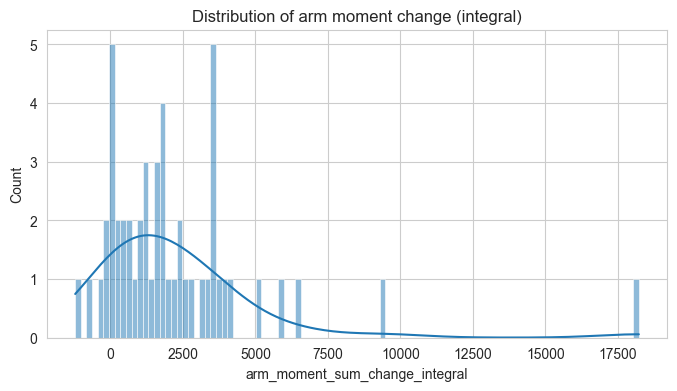
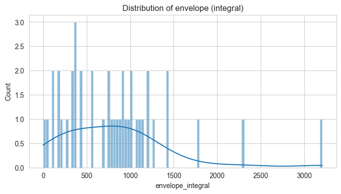
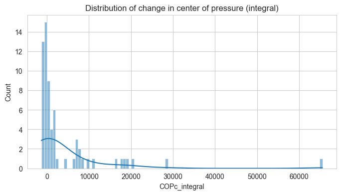
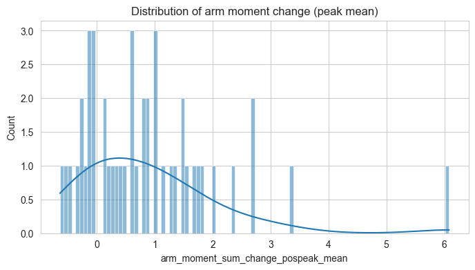
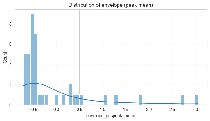
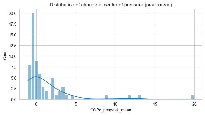
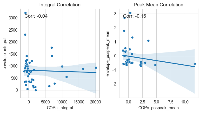
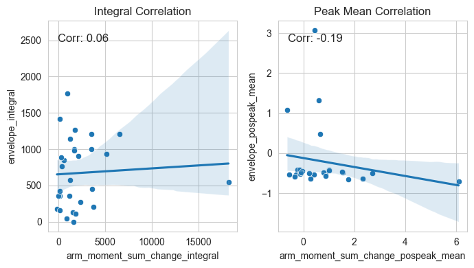
Let’s also have a first look on the distribution of our three measures of interest - arm moment (torque), COPc, and envelope.
These are for the features in cummulative form (integral)
These are for the features in instantaneous form (peak mean)
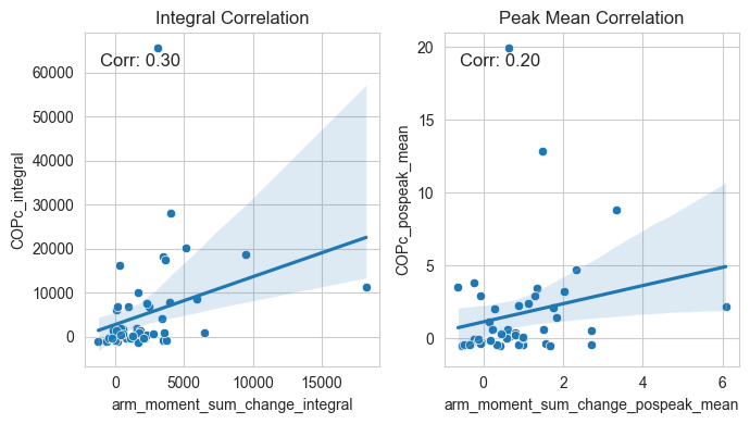
Lastly, let’s also look how are these three measures correlated with each other
Finally, because we will proceed with eXtreme Gradient Boosting per modality, we will also save the data separately for each modality.
# Separate data into three dfs based on modalityfeatures_df_gesture = features_df[features_df["modality"] =="gebaren"]features_df_combination = features_df[features_df["modality"] =="combinatie"]features_df_vocal = features_df[features_df["modality"] =="geluiden"]# Save themfeatures_df_gesture.to_csv(datafolder +"features_df_gesture.csv", index=False)features_df_combination.to_csv(datafolder +"features_df_combination.csv", index=False)features_df_vocal.to_csv(datafolder +"features_df_vocal.csv", index=False)
References
Berisha, Visar, Steven Sandoval, Rene Utianski, Julie Liss, and Andreas Spanias. 2014. “Characterizing the Distribution of the Quadrilateral Vowel Space Area.”The Journal of the Acoustical Society of America 135 (1): 421–27. https://doi.org/10.1121/1.4829528.
Daffertshofer, Andreas, Claudine J. C. Lamoth, Onno G. Meijer, and Peter J. Beek. 2004. “PCA in Studying Coordination and Variability: A Tutorial.”Clinical Biomechanics (Bristol, Avon) 19 (4): 415–28. https://doi.org/10.1016/j.clinbiomech.2004.01.005.
Hogan, Neville, and Dagmar Sternad. 2009. “Sensitivity of Smoothness Measures to Movement Duration, Amplitude, and Arrests.”Journal of Motor Behavior 41 (6): 529–34. https://doi.org/10.3200/35-09-004-RC.
Kadavá, Šárka, Aleksandra Ćwiek, Susanne Fuchs, and Wim Pouw. 2024. “What Do We Mean When We Say Gestures Are More Expressive Than Vocalizations? An Experimental and Simulation Study.”Proceedings of the Annual Meeting of the Cognitive Science Society 46 (0). https://escholarship.org/uc/item/2mp1v3v5.
Pouw, Wim, Mark Dingemanse, Yasamin Motamedi, and Aslı Özyürek. 2021. “A Systematic Investigation of Gesture Kinematics in Evolving Manual Languages in the Lab.”Cognitive Science 45 (7): e13014. https://doi.org/10.1111/cogs.13014.
Seth, Ajay, Jennifer L. Hicks, Thomas K. Uchida, Ayman Habib, Christopher L. Dembia, James J. Dunne, Carmichael F. Ong, et al. 2018. “OpenSim: Simulating Musculoskeletal Dynamics and Neuromuscular Control to Study Human and Animal Movement.”PLOS Computational Biology 14 (7): e1006223. https://doi.org/10.1371/journal.pcbi.1006223.
Trujillo, James, Irina Simanova, Harold Bekkering, and Asli Özyürek. 2018. “Communicative Intent Modulates Production and Comprehension of Actions and Gestures: A Kinect Study.”Cognition 180: 38–51. https://doi.org/10.1016/j.cognition.2018.04.003.
Xiong, Yingen, Francis Quek, and David Mcneill. 2002. “Hand Gesture Symmetric Behavior Detection and Analysis in Natural Conversation.” In, 179–84. https://doi.org/10.1109/ICMI.2002.1166989.
Yan, Yuke, James M. Goodman, Dalton D. Moore, Sara A. Solla, and Sliman J. Bensmaia. 2020. “Unexpected Complexity of Everyday Manual Behaviors.”Nature Communications 11 (1): 3564. https://doi.org/10.1038/s41467-020-17404-0.
Żywiczyński, Przemysław, Marek Placiński, Marta Sibierska, Monika Boruta-Żywiczyńska, Sławomir Wacewicz, Michał Meina, and Peter Gärdenfors. 2024. “Praxis, Demonstration and Pantomime: A Motion Capture Investigation of Differences in Action Performances.”Language and Cognition, 1–28. https://doi.org/10.1017/langcog.2024.8.