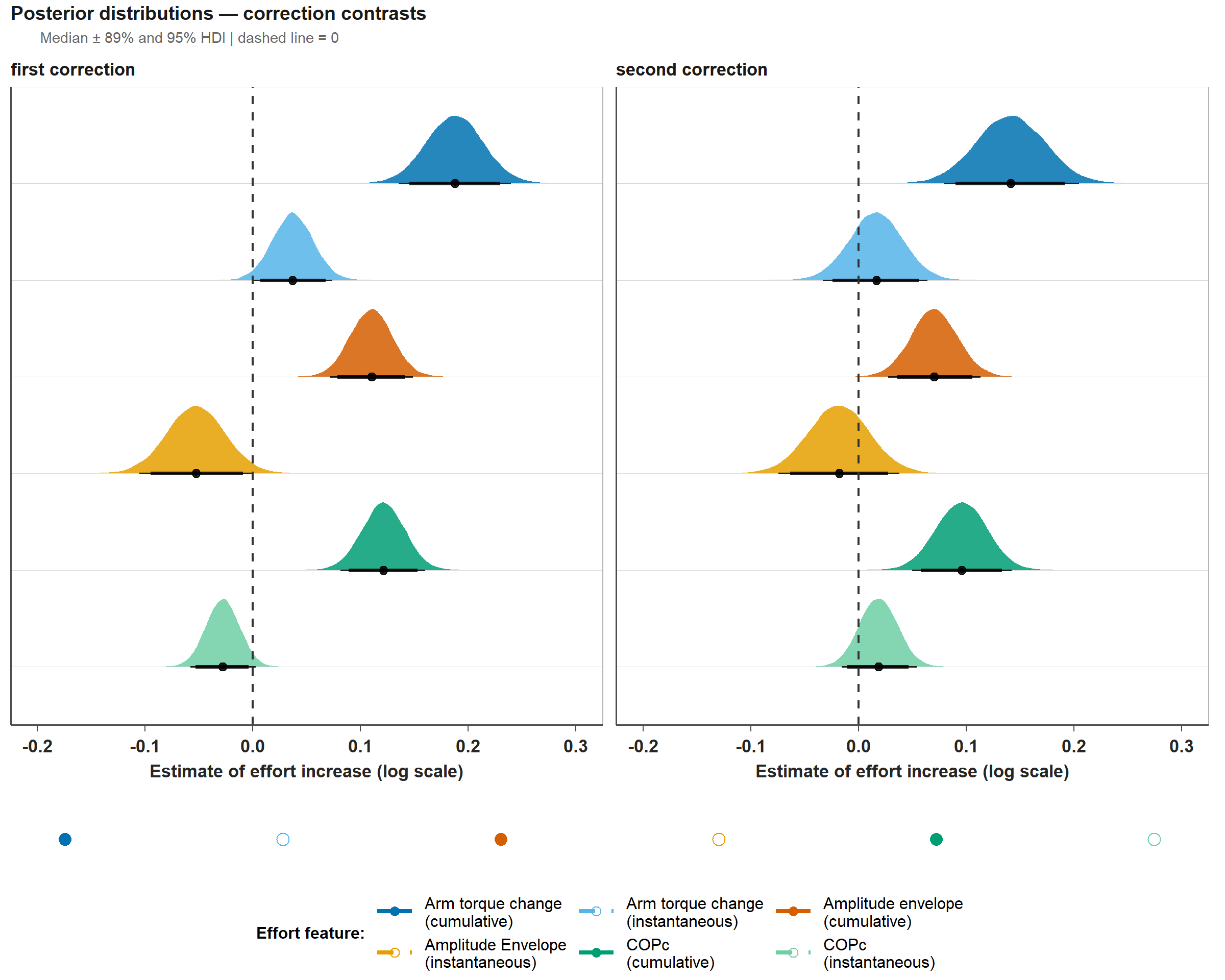
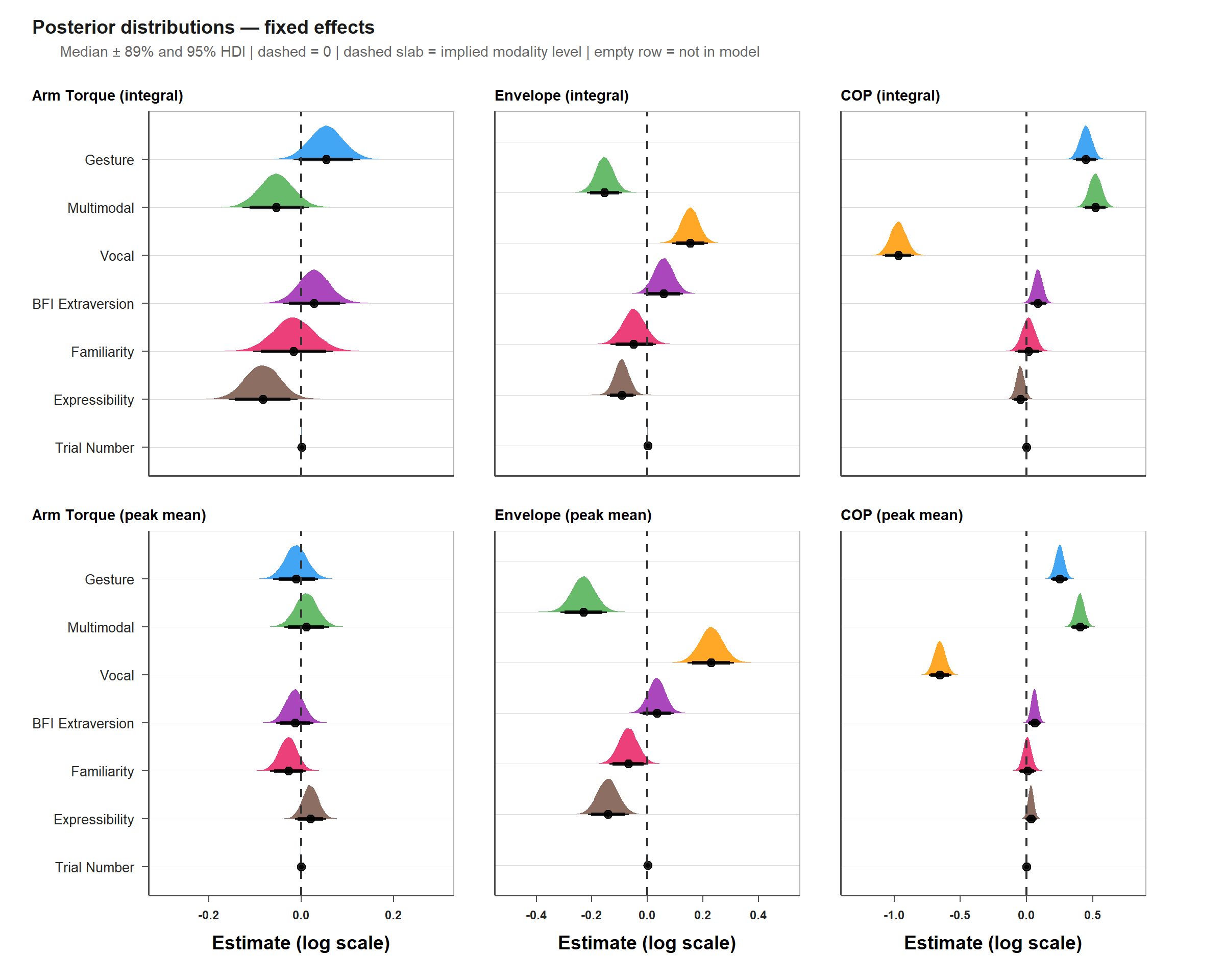
Modeling the effect of correction on physical effort

Overview

In this script, we are going to follow the pre-registered pipeline for modelling the relationship of effort and corrections. to confirm/reject our hypothesis.

These are:

H1: In corrections, people enhance some effort-related kinematic and/or acoustic features of their behavior relative to the baseline.

H2: The enhancement depends on similarity of the guesser’s answer and the original meaning. More similar answer will require/result in smaller enhancement (but still enhancement) than less similar answer.

The confirmatory analysis concerns six outcome variables, namely integral of torque change, integral of amplitude envelope, integral of change in center of pressure, and mean peak value of torque change, mean peak value of amplitude envelope, and mean peak value of change in center of pressure.

required_packages <- c("here",
                       "dplyr",
                       "tidyr",
                       "ggplot2",
                       "tidybayes",
                       "tibble",
                       "rcartocolor",
                       "patchwork",
                       "rstan",
                       "ggdag",
                       "dagitty",
                       "bayesplot",
                       "brms",
                       "bayestestR",
                       "tidyverse",
                       "emmeans",
                       "gt",
                       "ggtext")
                       
# Loop over the packages and check if they are installed
for (package in required_packages) {
  if (!require(package, character.only = TRUE)) {
    # If the package is not installed, install it
    install.packages(package)
    # Load the package
    library(package, character.only = TRUE)
  }
}


# brms setting
options(mc.cores = 4, brms.backend = 'cmdstanr', brms.file_refit = 'on_change')

# current folder (first go to session -> set working directory -> to source file location)
curfolder     <- getwd()
parentfolder  <- dirname(curfolder)
featurefolder <- paste0(parentfolder, '/05_TS_featureExtraction/Datasets/')
rawfolder     <- paste0(parentfolder, '/00_raw/')
datasets      <- paste0(curfolder, '/datasets/')
models        <- paste0(curfolder, '/models/')
plots         <- paste0(curfolder, '/plots/')
summaries     <- paste0(curfolder, '/summaries/')

source(here(curfolder, "R-helper.R"))

Loading in our data

This is the feature dataframe we will be using. It contains all features colected in previous script, together with demographic information about the participants. For confirmatory analysis, we will need only 6 features - arm torque integral, arm torque peak mean, COPc integral, COPc peak mean, envelope integral and envelope peak mean from the data_feat. From demographics, we will need only BFI and Familiarity

# This is the relevant df
data_feat <- read_csv(paste0(featurefolder, "features_df_nonzscored_final_with_demo.csv"))

# This is for demographics overview
data_demo <- read_csv(paste0(rawfolder, "all_demodata.csv"))

featstokeep <- c('COPc_peak_mean', 'envelope_norm_peak_mean', 'arm_moment_sum_change_peak_mean', 'COPc_integral', 'envelope_norm_integral', 'arm_moment_sum_change_integral', 'correction', 'concept', 'TrialID', 'modality', 'expressibility', 'answer_prev', 'answer_prev_dist', 'answer_fol', 'answer_fol_dist', 'pcn_ID', 'BFI_extra', 'BFI_agree', 'BFI_consc', 'BFI_negemo', 'BFI_open', 'Familiarity', 'duration_trial')

# We will merge again correction c0 and c0_only because we are not interested in the difference between these two in our main question
data_feat$correction <- sapply(strsplit(as.character(data_feat$correction_info), "_"), `[`, 1)

# Subset the dataframe
data_feat <- data_feat %>% select(all_of(featstokeep))

# Create column TrialNumber by extracting third element from TrialID
data_feat$TrialNumber <- sapply(strsplit(data_feat$TrialID, "_"), function(x) x[3])

# Create column SessionID to track dyad
data_feat$SessionID <- sapply(strsplit(data_feat$TrialID, "_"), function(x) x[1])

knitr::kable(head(data_feat, 15))

COPc_peak_mean	envelope_norm_peak_mean	arm_moment_sum_change_peak_mean	COPc_integral	envelope_norm_integral	arm_moment_sum_change_integral	correction	concept	TrialID	modality	expressibility	answer_prev	answer_prev_dist	answer_fol	answer_fol_dist	pcn_ID	BFI_extra	BFI_agree	BFI_consc	BFI_negemo	BFI_open	Familiarity	duration_trial	TrialNumber	SessionID
1.09759	0.27932	20.08211	2521.490	354.71586	34093.02	c1	grommen	10_2_100_p1	vocal	0.751	tijger	0.13702	leeuw	0.10809	10_p1	0.1638325	0.1949416	0.4364203	0.1371162	0.3072000	12	5156	100	10
0.93058	0.37726	12.69215	2881.611	633.11275	32330.70	c2	grommen	10_2_101_p1	vocal	0.751	leeuw	0.10809	grommen	1.00000	10_p1	0.1638325	0.1949416	0.4364203	0.1371162	0.3072000	12	5948	101	10
0.56922	0.13287	14.01212	1440.953	272.90953	52290.18	c1	lopen	10_2_103_p1	vocal	0.319	wandelen	0.75055	tikken	0.25607	10_p1	0.1638325	0.1949416	0.4364203	0.1371162	0.3072000	12	6208	103	10
0.77717	0.12505	19.45120	3739.410	490.76049	46241.13	c0	fluisteren	10_2_104_p1	vocal	0.703	NA	NA	fluisteren	1.00000	10_p1	0.1638325	0.1949416	0.4364203	0.1371162	0.3072000	12	10066	104	10
1.06165	0.02226	9.87082	4700.776	315.61850	43817.87	c0	langzaam	10_2_10_p0	gesture	0.689	NA	NA	slowmotion	0.80670	10_p0	-0.1226291	-0.8927582	-0.0682717	-0.1085153	0.7124818	13	14816	10	10
1.10174	0.02125	29.80697	2897.690	110.35390	41955.64	c2	langzaam	10_2_12_p0	gesture	0.689	joggen	0.22412	langzaam	1.00000	10_p0	-0.1226291	-0.8927582	-0.0682717	-0.1085153	0.7124818	13	5204	12	10
0.65393	0.02199	25.26511	1364.247	94.67007	48342.93	c0	weten	10_2_13_p0	gesture	0.507	NA	NA	denken	0.63104	10_p0	-0.1226291	-0.8927582	-0.0682717	-0.1085153	0.7124818	13	4442	13	10
0.84991	0.02174	31.60588	1020.479	62.42853	26617.72	c1	weten	10_2_14_p0	gesture	0.507	denken	0.63104	idee	0.29182	10_p0	-0.1226291	-0.8927582	-0.0682717	-0.1085153	0.7124818	13	2926	14	10
0.61721	0.02214	44.06453	1089.807	94.30230	44307.83	c2	weten	10_2_15_p0	gesture	0.507	idee	0.29182	bedenken	0.51304	10_p0	-0.1226291	-0.8927582	-0.0682717	-0.1085153	0.7124818	13	4422	15	10
1.28804	0.03341	20.45161	2726.329	161.04506	70782.63	c0	zwaar	10_2_21_p1	gesture	0.689	NA	NA	zwanger	0.10441	10_p1	0.1638325	0.1949416	0.4364203	0.1371162	0.3072000	12	4866	21	10
1.67104	0.03369	21.55195	8373.810	353.80893	157838.42	c1	zwaar	10_2_22_p1	gesture	0.689	zwanger	0.10441	dik	0.59389	10_p1	0.1638325	0.1949416	0.4364203	0.1371162	0.3072000	12	10690	22	10
1.58215	0.03535	18.36742	4388.624	219.71219	64983.11	c2	zwaar	10_2_23_p1	gesture	0.689	dik	0.59389	zwaar	1.00000	10_p1	0.1638325	0.1949416	0.4364203	0.1371162	0.3072000	12	6618	23	10
1.22581	0.03452	23.06106	1841.308	126.24706	110313.48	c0	niet	10_2_24_p1	gesture	0.546	NA	NA	kruis	0.00506	10_p1	0.1638325	0.1949416	0.4364203	0.1371162	0.3072000	12	3804	24	10
1.23902	0.03491	46.16350	3127.201	160.58531	198559.45	c1	niet	10_2_25_p1	gesture	0.546	kruis	0.00506	verboden	0.36632	10_p1	0.1638325	0.1949416	0.4364203	0.1371162	0.3072000	12	4842	25	10
1.00259	0.03363	19.55126	2329.973	174.37028	68083.24	c2	niet	10_2_26_p1	gesture	0.546	verboden	0.36632	luisteren	0.01263	10_p1	0.1638325	0.1949416	0.4364203	0.1371162	0.3072000	12	5256	26	10

Basic statistics

These are some basic statistics regarding our participant pool

[1] "---- DEMOGRAPHICS ----"

[1] "Number of participants: 122"

[1] "Number of dyads: 61"

[1] "Gender distribution:"

[1] "anders: 1, man: 20, non-binair: 1, vrouw: 98, zeg ik liever niet: 1"

[1] "Mean Age: 19.9917355371901"

[1] "Age range: 17 - 27"

[1] "Handedness distribution:"

[1] "L: 14, R: 107"

[1] "---- TRIALS ----"

[1] "Number of trials per modality:"

[1] "gesture: 1256, multimodal: 1262, vocal: 1952"

[1] "Number of trials per correction:"

[1] "c0: 2220, c1: 1324, c2: 926"

# A tibble: 9 × 3
  modality   correction     n
  <chr>      <chr>      <int>
1 gesture    c0           702
2 gesture    c1           352
3 gesture    c2           202
4 multimodal c0           708
5 multimodal c1           354
6 multimodal c2           200
7 vocal      c0           810
8 vocal      c1           618
9 vocal      c2           524

H1: Stating causal model

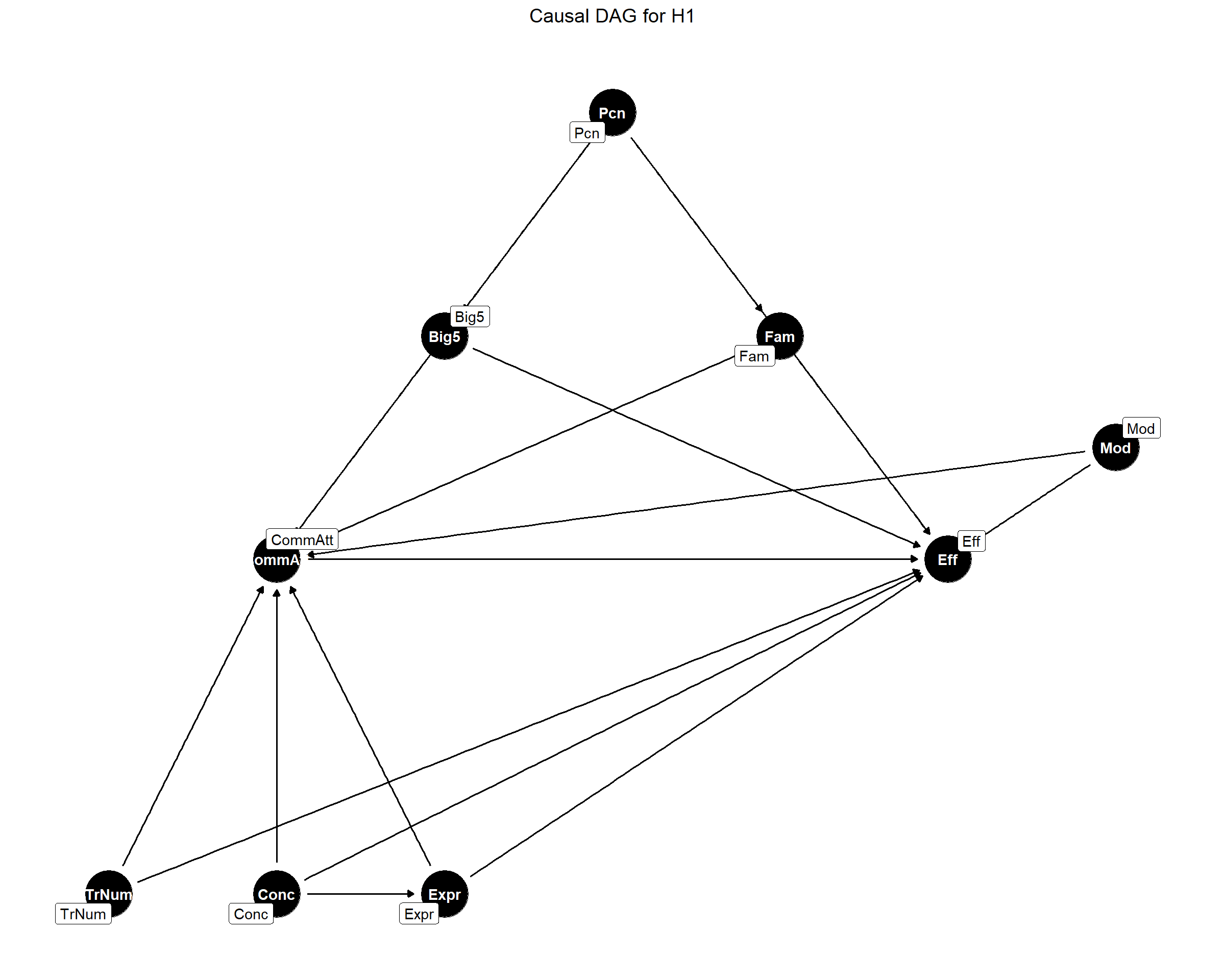
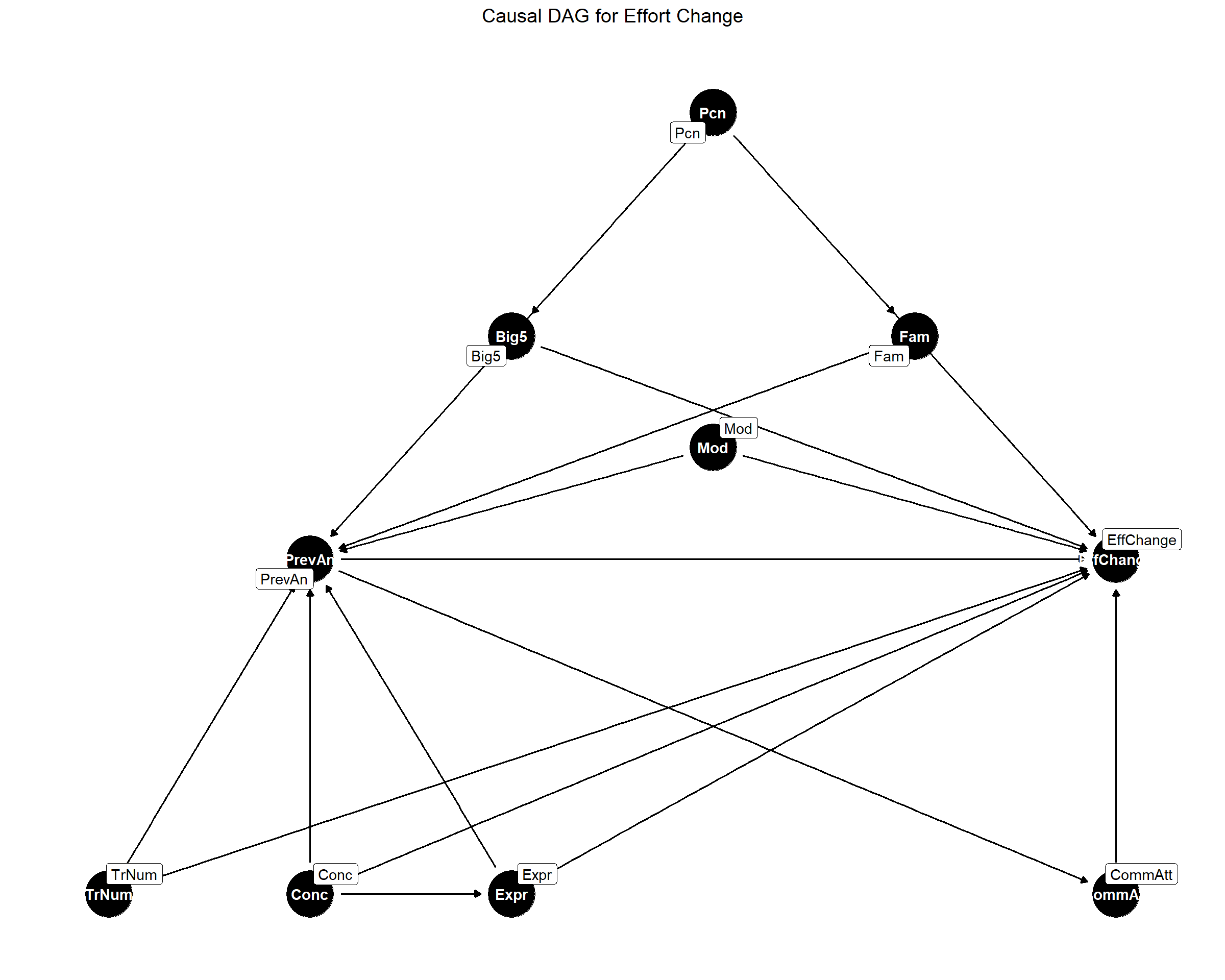
Before simulating synthetic data, we will first formulate our causal model to explicitly identify common causes, and hence prevent (or rather minimize) confounding in our statistical model. Note that while we are interested in causal relationship between effort (outcome) and communicative attempt (predictor for H1) and answer similarity (predictor for H2), we need to acknowledge that there are other factors possibly contributing to the outcome variable, despite the experiment beling relatively controlled. These relate, for instance, to the participants (e.g., personality traits) or stimuli (i.e., concepts). Our causal model therefore includes more variables that are identified as potentially sharing causal path with our primary predictor - communicative attempt. They are not of primary interest, they ensure we can isolate the causal effect of the main predictor on the outcome variable - effort.

To explicitly formulate the causal paths, we will start our analysis visualizing our causal model using directed acyclic graph (DAG). We will use packages dagitty and ggdag to create these DAGs and to extract implied independencies and adjustment set. DAG will help us clarify the causal model and introduce the predictors we aim to model (McElreath, 2018). This model goes hand in hand with the logic underlying the synthetic data we create below.

Our first hypothesis goes as follows:

H1: Correction recruits more physical effort than the baseline performance.

The relationship of interest is the causal effect of communicative attempt on effort. Further, our causal model includes following assumptions:

• Personality traits (measured with BFI) will influence effort (e.g., people are more willing to put more effort if they are open-minded) and also communicative attempt (e.g., more extroverted people are better in this game, therefore they need less attempts)

• Familiarity with guessing partner influences effort (ditto) as well as communicative attempt (e.g., friends are better in this game than strangers)

• Similarly, participant will also directly influence effort and commAtt, because personality traits might not be capturing all variation

• Expressibility of concepts is going to influence effort (e.g., more expressible concepts allow more enhancement - but could be also other direction) as well as CommAtt (e.g., more expressible concepts are more readily guessed and don’t need more attempts)

• Similarly, concept will also directly influence effort and commAtt, because expressibility might not be capturing all variation

• Modality (uni vs. multi) will influence the value of effort. We assume that in unimodal condition, the feature does not need to account for synergic relations with the other modality, and may carry the whole signal. In multimodal condition, however, there may be synergic relations that moderate the full expressiveness of this feature

• Trial number (characterising how far one is in the experiment) could be hinting on learning processes through out the experiment, or - the other direction - on increasing fatigue

Note that we are aware that some of the parameters might be correlated and we might run into issues with collinearity. While DAG does not help to solve it, it does help in detecting whether the two potentially highly correlated variables have separate causal effect or share a common cause. If they share common cause, there might be a problem in distinguishing their effects from each other. We will report inter-variable correlations when analyzing the actual data.

Causal DAG for H1

These are the implied conditional independencies

Big5 _||_ Conc
Big5 _||_ Expr
Big5 _||_ Fam | Pcn
Big5 _||_ Mod
Big5 _||_ TrNm
Conc _||_ Fam
Conc _||_ Mod
Conc _||_ Pcn
Conc _||_ TrNm
Expr _||_ Fam
Expr _||_ Mod
Expr _||_ Pcn
Expr _||_ TrNm
Fam _||_ Mod
Fam _||_ TrNm
Mod _||_ Pcn
Mod _||_ TrNm
Pcn _||_ TrNm

This is the adjustment set that needs to be included in the model to make sure we are not confounding

{ Big5, Conc, Expr, Fam, Mod, Pcn, TrNum }

H1: Modelling

In this part, we are going to test the following hypothesis:

H1: Correction recruits more physical effort than the baseline performance.

We will fit Bayesian mixed effect models using brms package (Bürkner, 2017).

TORQUE

Data wrangling

To be able to interpret the data, we will first need to do some data wrangling

# Get rid of vocal modality (torque is relevant only for gesture-only and multimodal condition)
df_ges <- data_feat |> filter(modality != 'vocal')

# CC modality
df_ges$modality <- factor(df_ges$modality,
                          levels = c('gesture', 'multimodal'))
contrasts(df_ges$modality) <- contr.sum(2)/2

df_ges$TrialNumber <- as.numeric(df_ges$TrialNumber)  # Ensure TrialNumber is numeric
df_ges$TrialNumber_c <- df_ges$TrialNumber - median(range(df_ges$TrialNumber)) # Center trial number

# The rest as factor
df_ges$correction <- as.factor(df_ges$correction)
df_ges$pcn_ID <- as.factor(df_ges$pcn_ID)
df_ges$concept <- as.factor(df_ges$concept)
df_ges$SessionID <- as.factor(df_ges$SessionID)

# Contrast-coding of categorical variables - correction
df_ges$correction <- factor(df_ges$correction, 
                                   levels = c('c0', 'c1', 'c2'))
contrasts(df_ges$correction) <- MASS::contr.sdif(3) 

# Z-score familiarity to be compatible with BFI
df_ges$Familiarity <- scale(df_ges$Familiarity, center = TRUE, scale = TRUE) |> as.numeric()

# Z-score expressibility within modality
df_ges <-
  df_ges |>
  group_by(modality) |>
  mutate(expressibility_z = (expressibility - mean(expressibility))/ sd(df_ges$expressibility, na.rm = T)) |>
  ungroup()

Note: BFI has been z-scored when processing metadata as this is the common procedure for calculating each trait’s score

Note

This is how correction is contrast-coded:

      2-1        3-2

c0 -0.6666667 -0.3333333 c1 0.3333333 -0.3333333 c2 0.3333333 0.6666667

This should be enough given that we are interested in the incrementals.

This is how modality is cc-ed:

       [,1]

gesture 0.5 multimodal -0.5

Cummulative torque

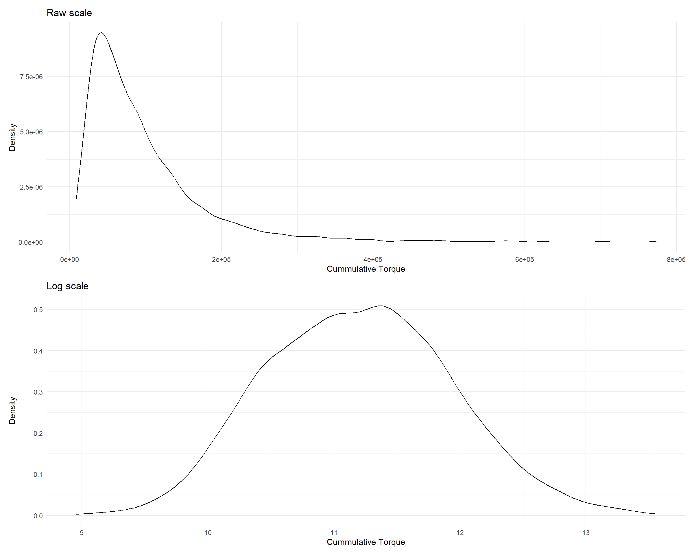
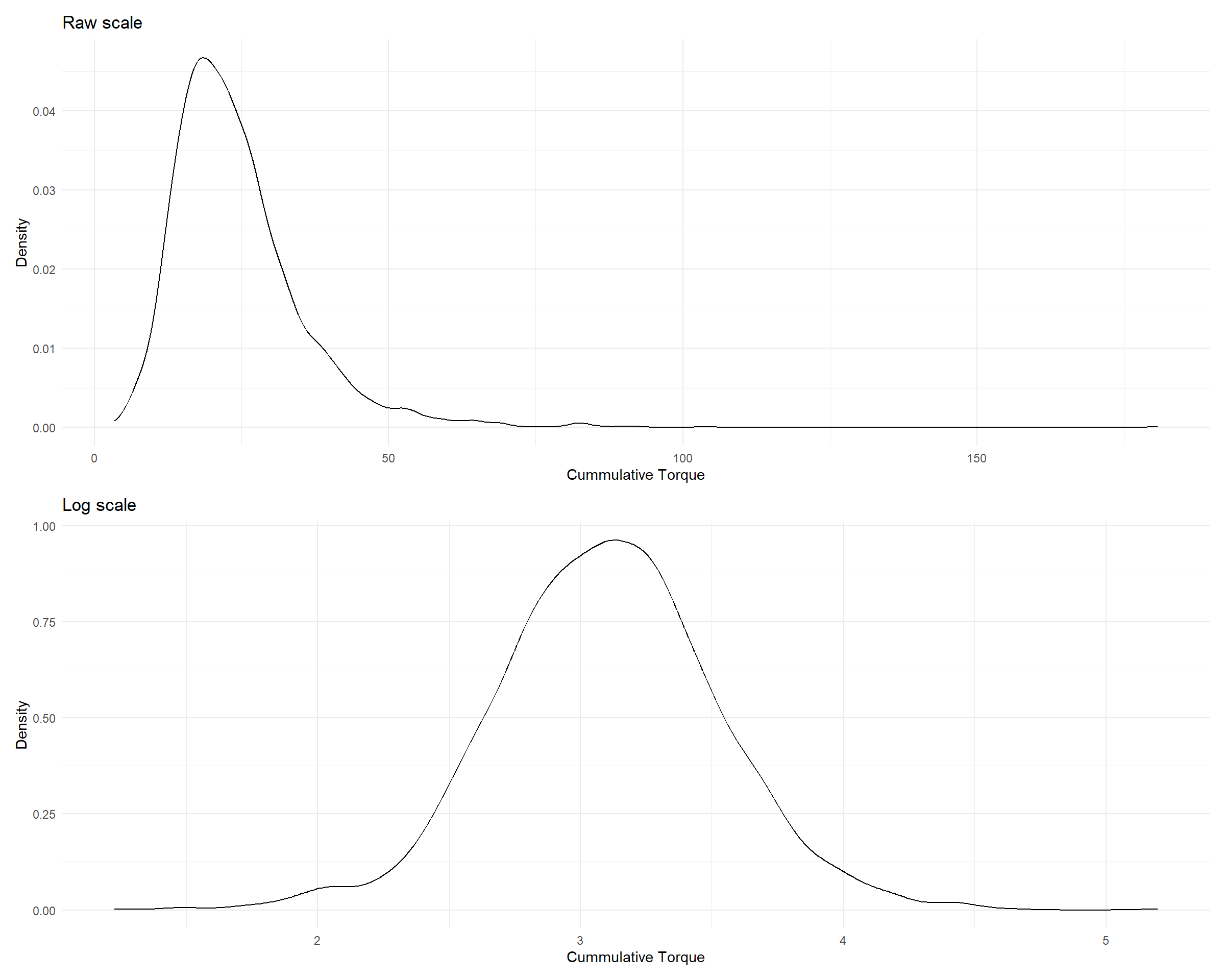
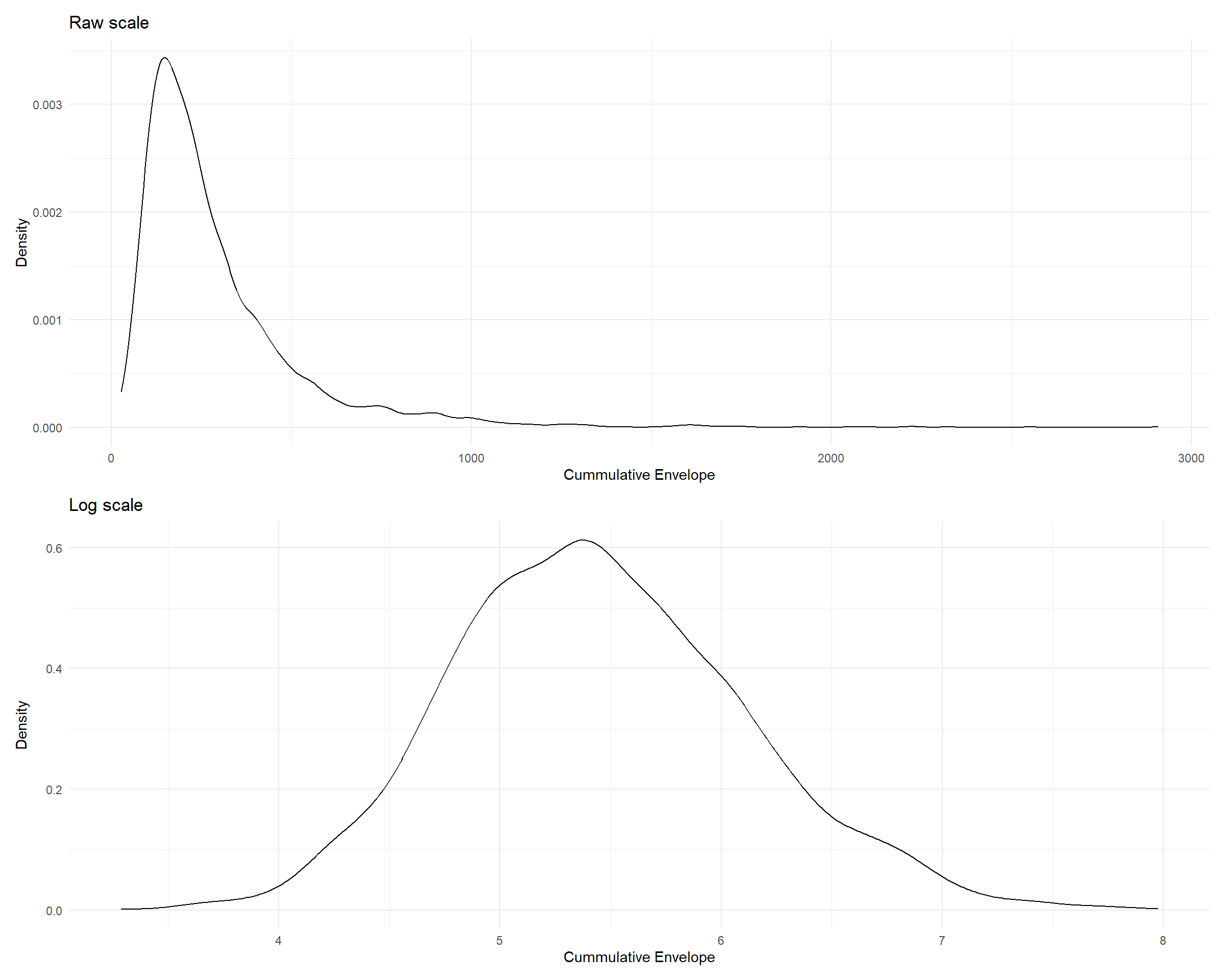
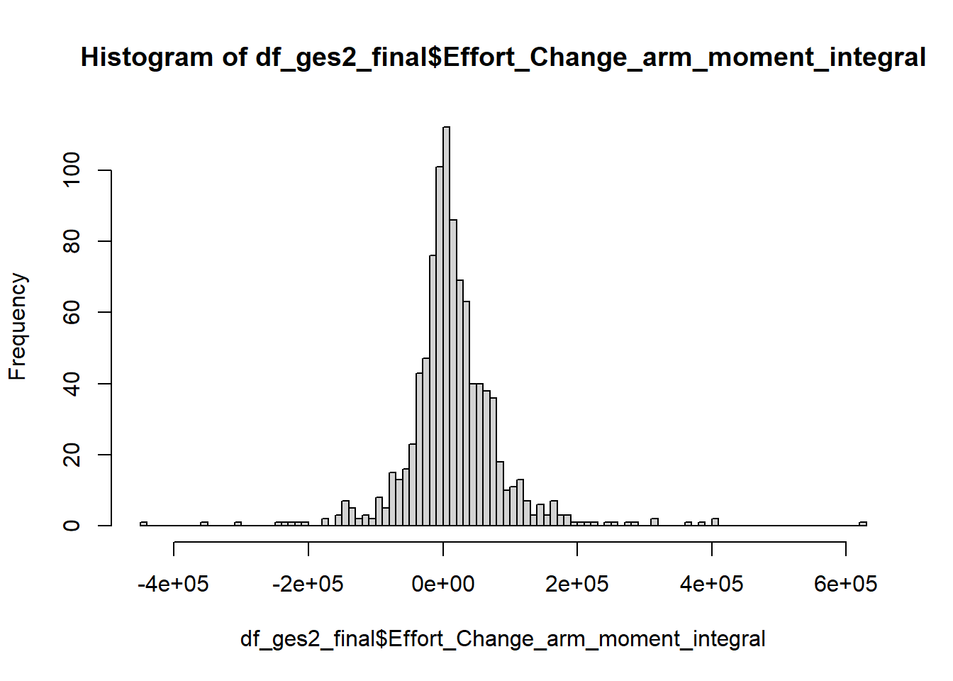
This is how cumulative torque is distributed (raw values and log-transformed)

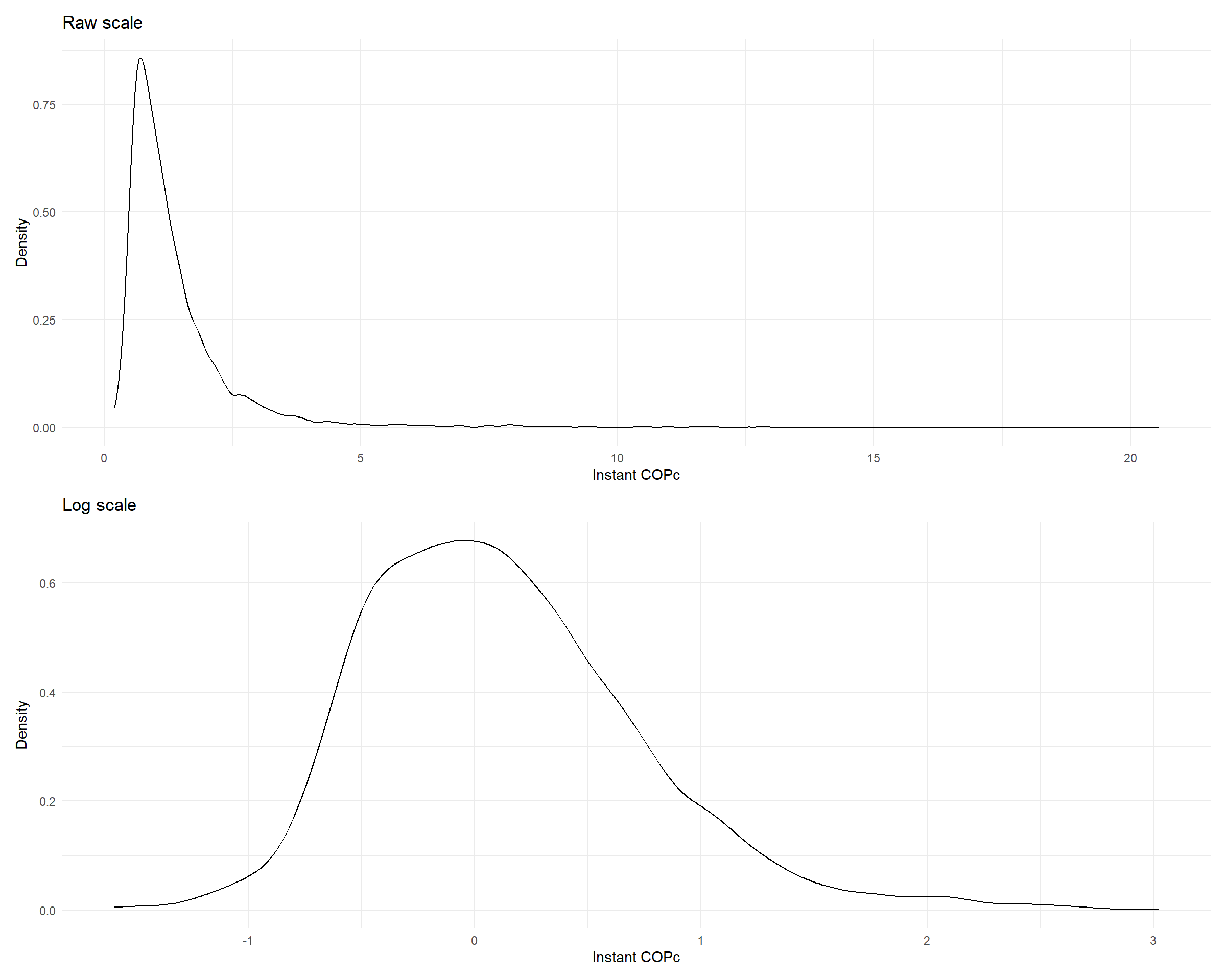
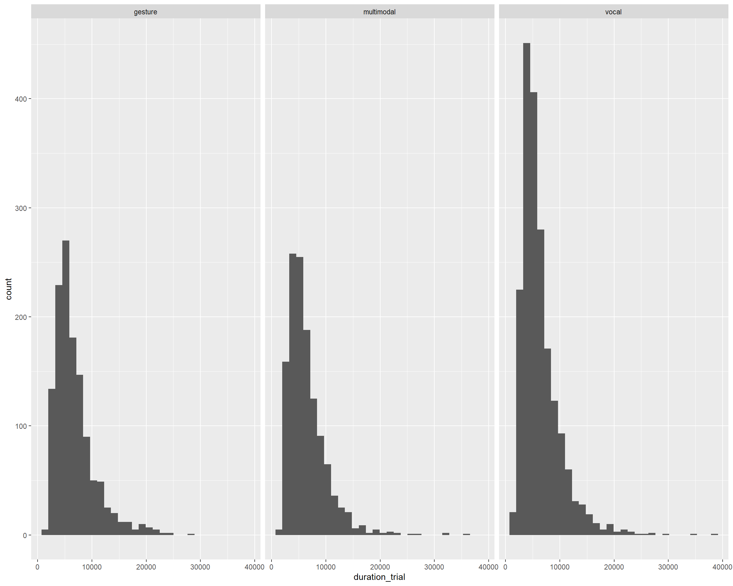
Distribution of cumulative torque

The plot points to log-normal distribution, which we will also use as our family.

Model 0 - Intercept only

In the preregistration, we layed out a workflow for fitting the desired models. We will now fit only two models from all: intercept-only model and model that reproduces DAG (with varying slopes and intercepts for concept, participant and dyad).

We will also add weakly informative priors based on reasonable ranges that limit extreme values. We will set them as follows:

• Intercept: The geometric mean of arm moment for the reference group is most plausibly around exp(11) ≈ 6,000 raw units, but we allow considerable uncertainty — 95% of prior mass spans exp(7) to exp(15)

• correction: We have no prior expectation of whether corrections increase or decrease effort. But we allow each correction step to plausibly up to nearly triple (×2.7) or halve (×0.37) arm moment. Effects larger than that are considered implausible.

priors_h1m0_torq_cum <- c(
  set_prior("normal(11, 2)", class = "Intercept"),
  set_prior("normal(0, 0.5)", class = "sigma"),
  set_prior("normal(0,0.5)", class = "b", coef = "correction2M1"),
  set_prior("normal(0,0.5)", class = "b", coef = "correction3M2")
)


if (file.exists(here(models, "h1.m0_torq_cum.rds"))){
  
  h1.m0_torq_cum <- readRDS(here(models, "h1.m0_torq_cum.rds"))
  h1.m0_torq_cum_R2 <- readRDS(here(models, "h1.m0_torq_cum_R2.rds"))
  
} else {
  h1.m0_torq_cum <- brm(arm_moment_sum_change_integral ~ 1 + correction, 
                  data = df_ges,
                  family = lognormal(),
                  prior = priors_h1m0_torq_cum,
                  iter = 2000,
                  cores = 4,
                  seed = 0209)
  
  # Add criterions for later diagnostics
  h1.m0_torq_cum <- add_criterion(h1.m0_torq_cum, criterion = c("loo", "waic"))
  
  # Calculate also variance explained (R^2)
  h1.m0_torq_cum_R2 <- bayes_R2(h1.m0_torq_cum)
  
  # Save both as objects
  saveRDS(h1.m0_torq_cum, here(models, "h1.m0_torq_cum.rds"))
  saveRDS(h1.m0_torq_cum_R2, here(models, "h1.m0_torq_cum_R2.rds"))

}

# Summary
summary(h1.m0_torq_cum)

 Family: lognormal 
  Links: mu = identity 
Formula: arm_moment_sum_change_integral ~ 1 + correction 
   Data: df_ges (Number of observations: 2495) 
  Draws: 4 chains, each with iter = 2000; warmup = 1000; thin = 1;
         total post-warmup draws = 4000

Regression Coefficients:
              Estimate Est.Error l-95% CI u-95% CI Rhat Bulk_ESS Tail_ESS
Intercept        11.27      0.02    11.24    11.30 1.00     3820     3317
correction2M1     0.20      0.03     0.13     0.27 1.00     3157     3080
correction3M2     0.14      0.05     0.05     0.23 1.00     3025     2974

Further Distributional Parameters:
      Estimate Est.Error l-95% CI u-95% CI Rhat Bulk_ESS Tail_ESS
sigma     0.72      0.01     0.70     0.74 1.00     3742     2812

Draws were sampled using sample(hmc). For each parameter, Bulk_ESS
and Tail_ESS are effective sample size measures, and Rhat is the potential
scale reduction factor on split chains (at convergence, Rhat = 1).

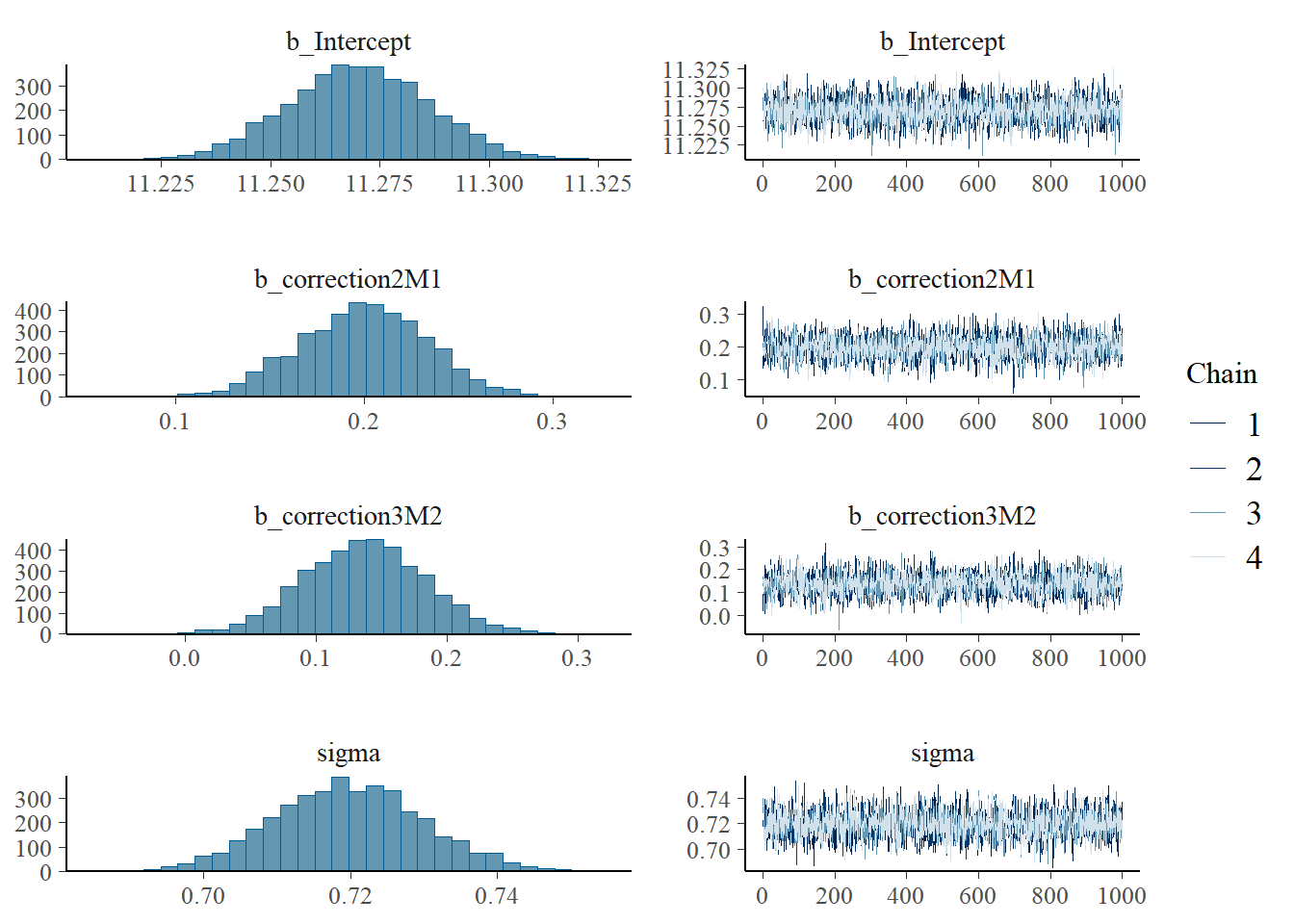
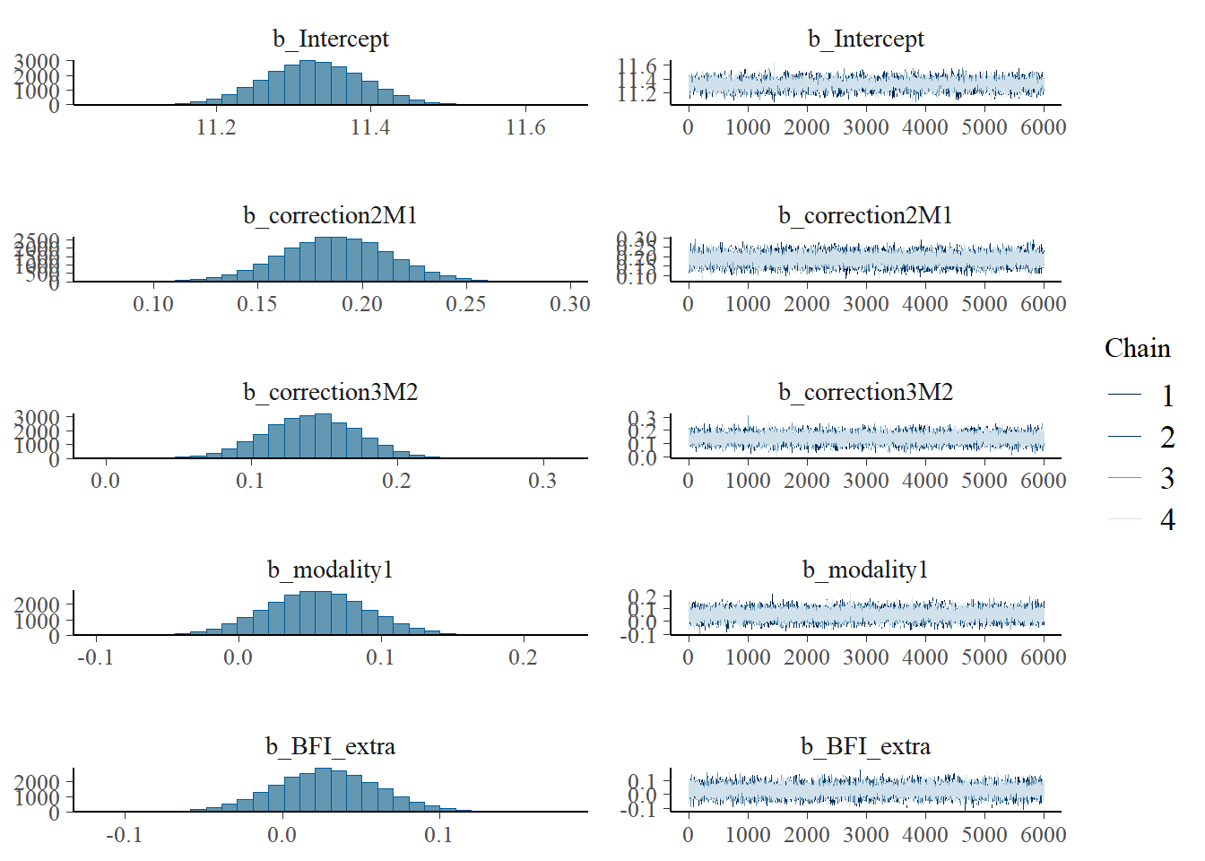
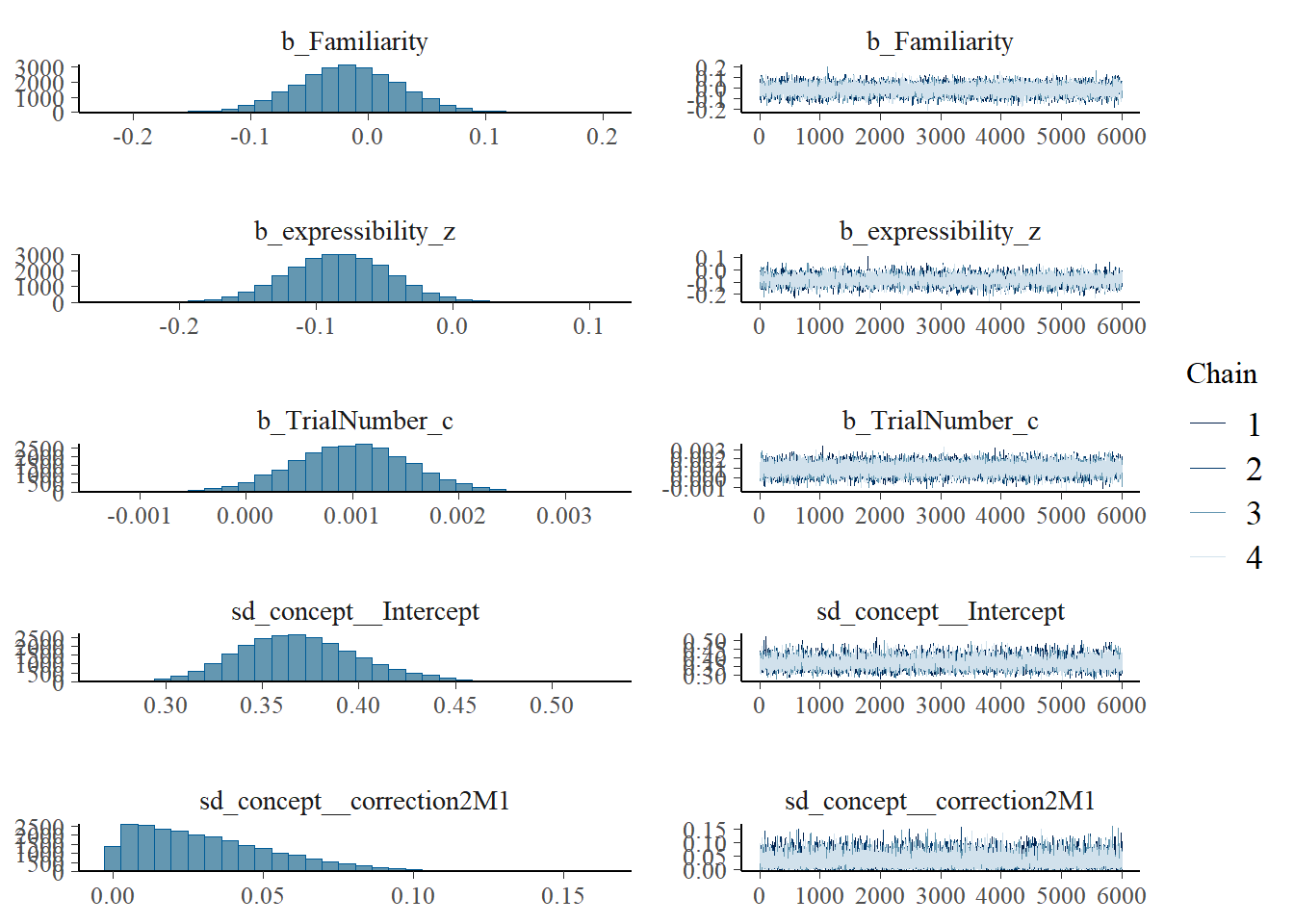
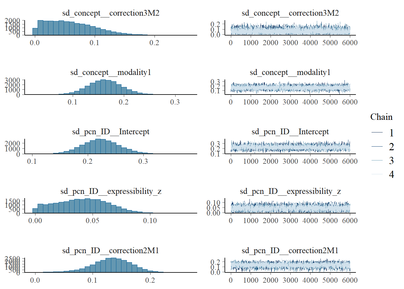
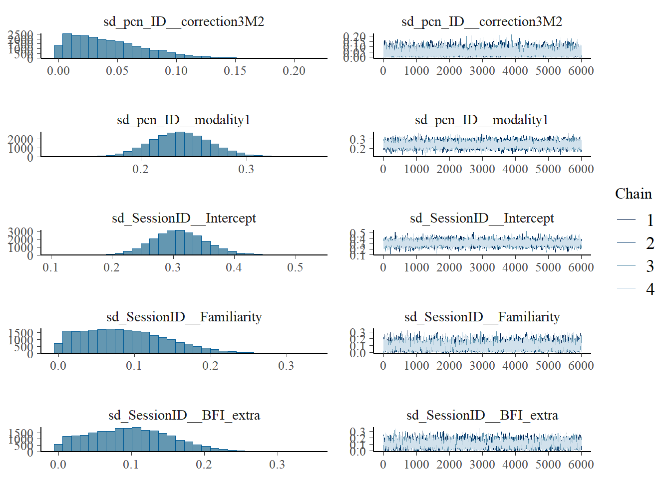
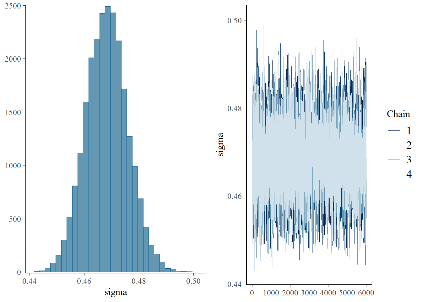
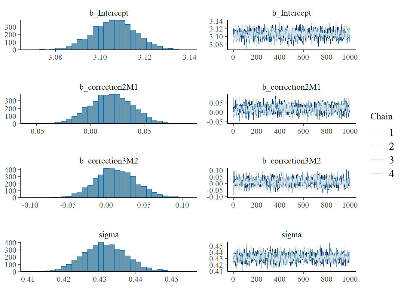
First let’s check whether all chains are healthy

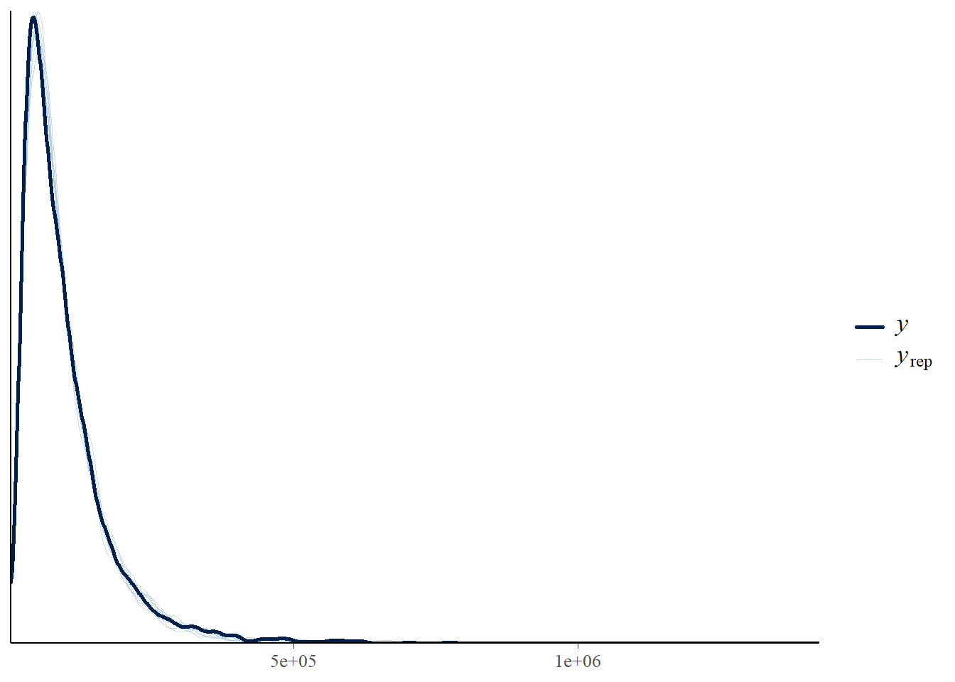
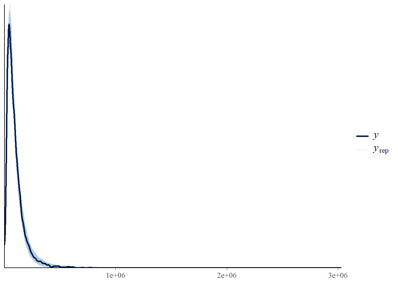
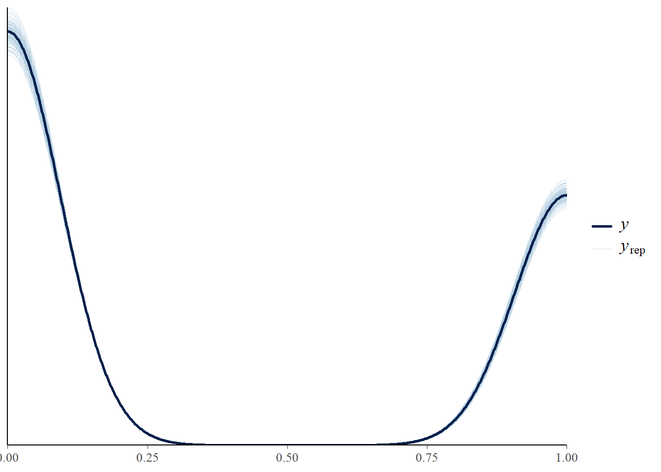
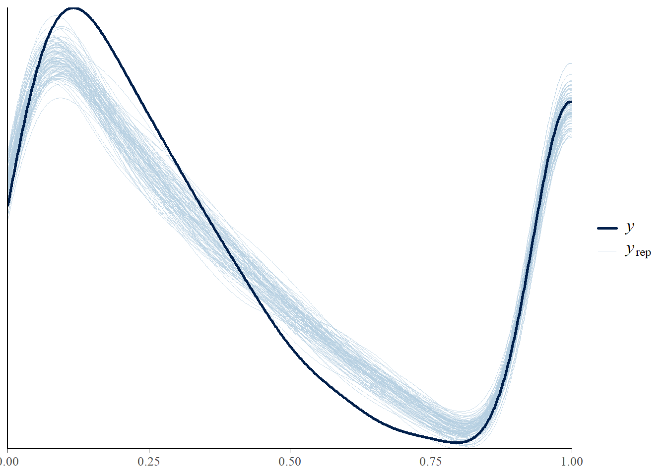
… whether predicted values are close to the raw distribution

… and what is the residual error

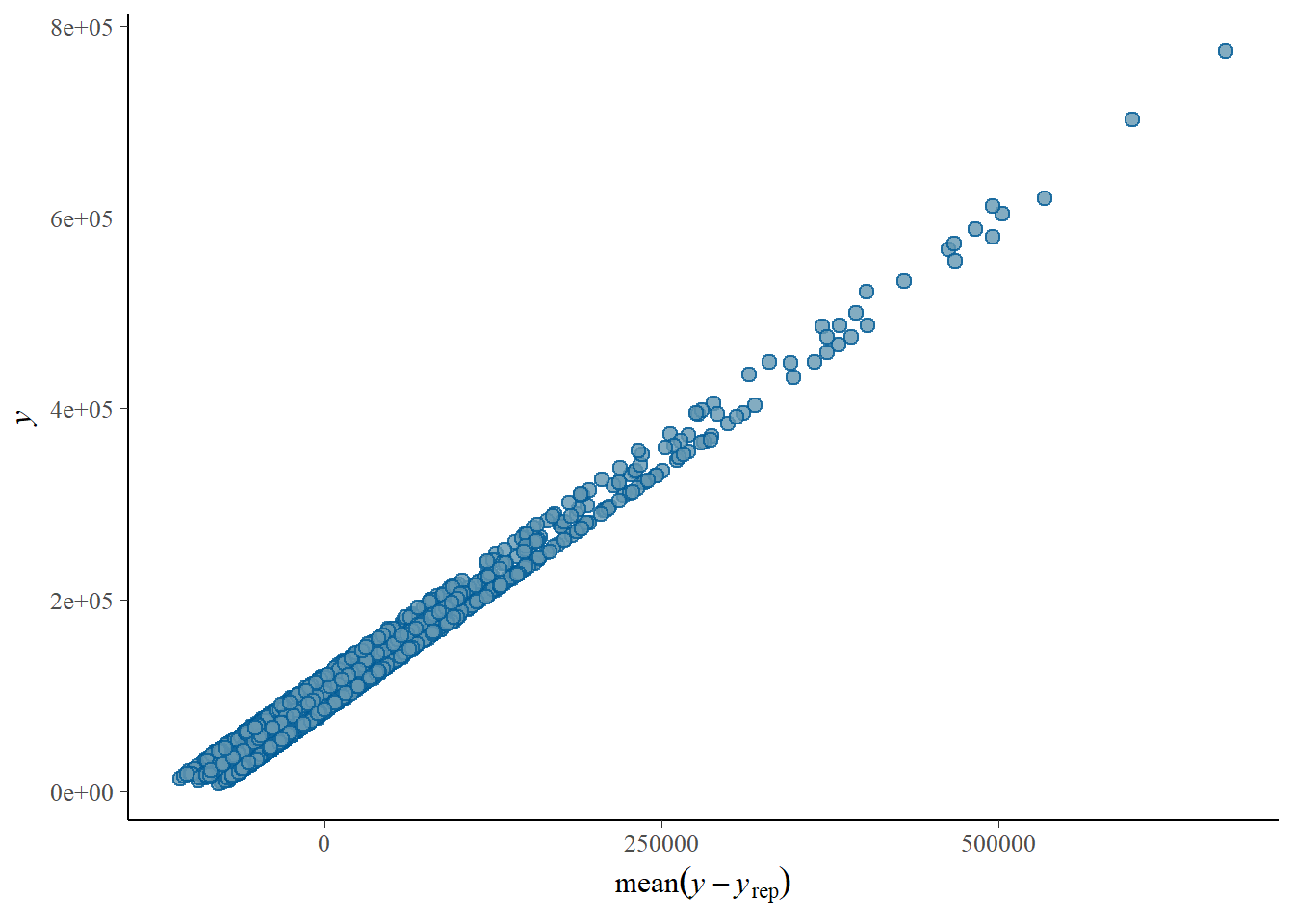
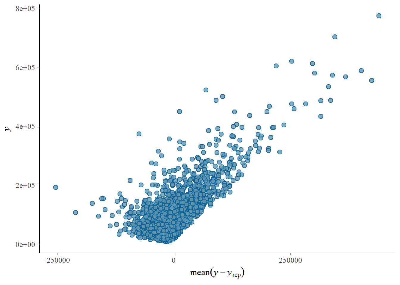
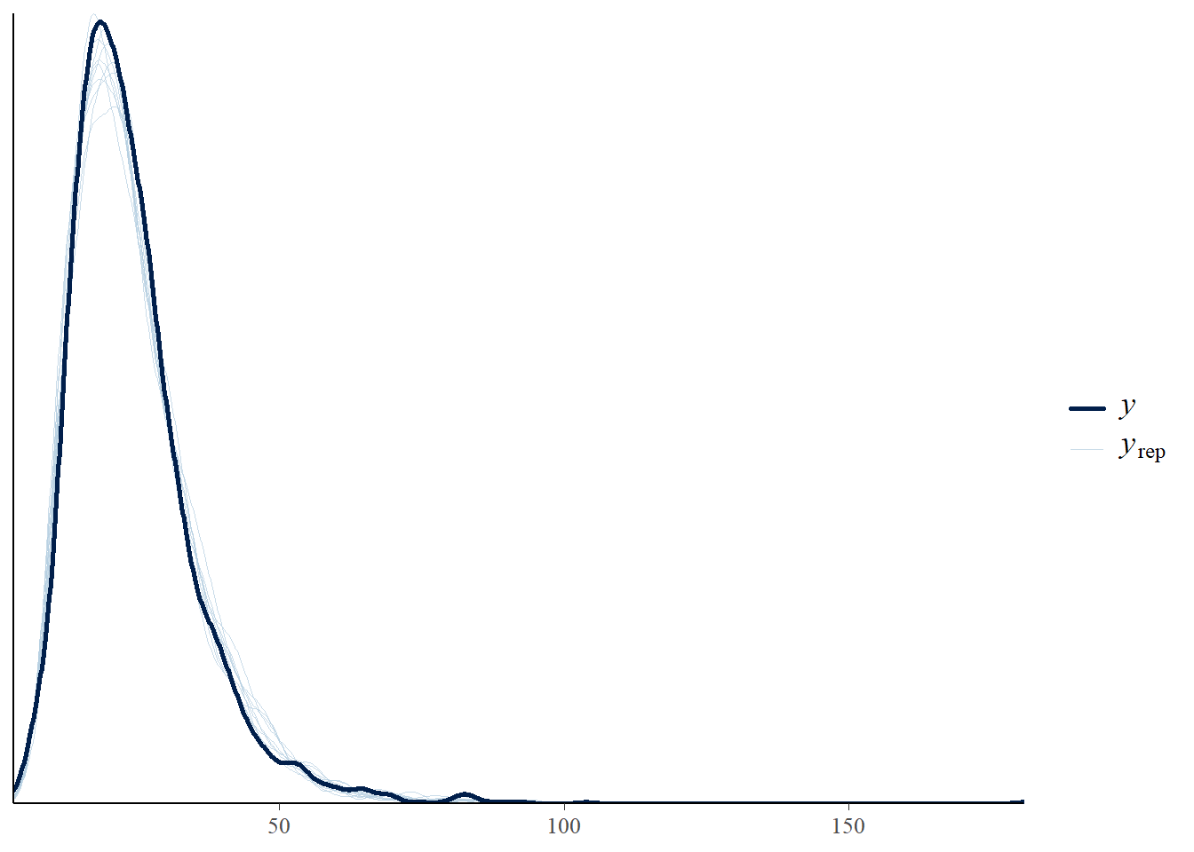
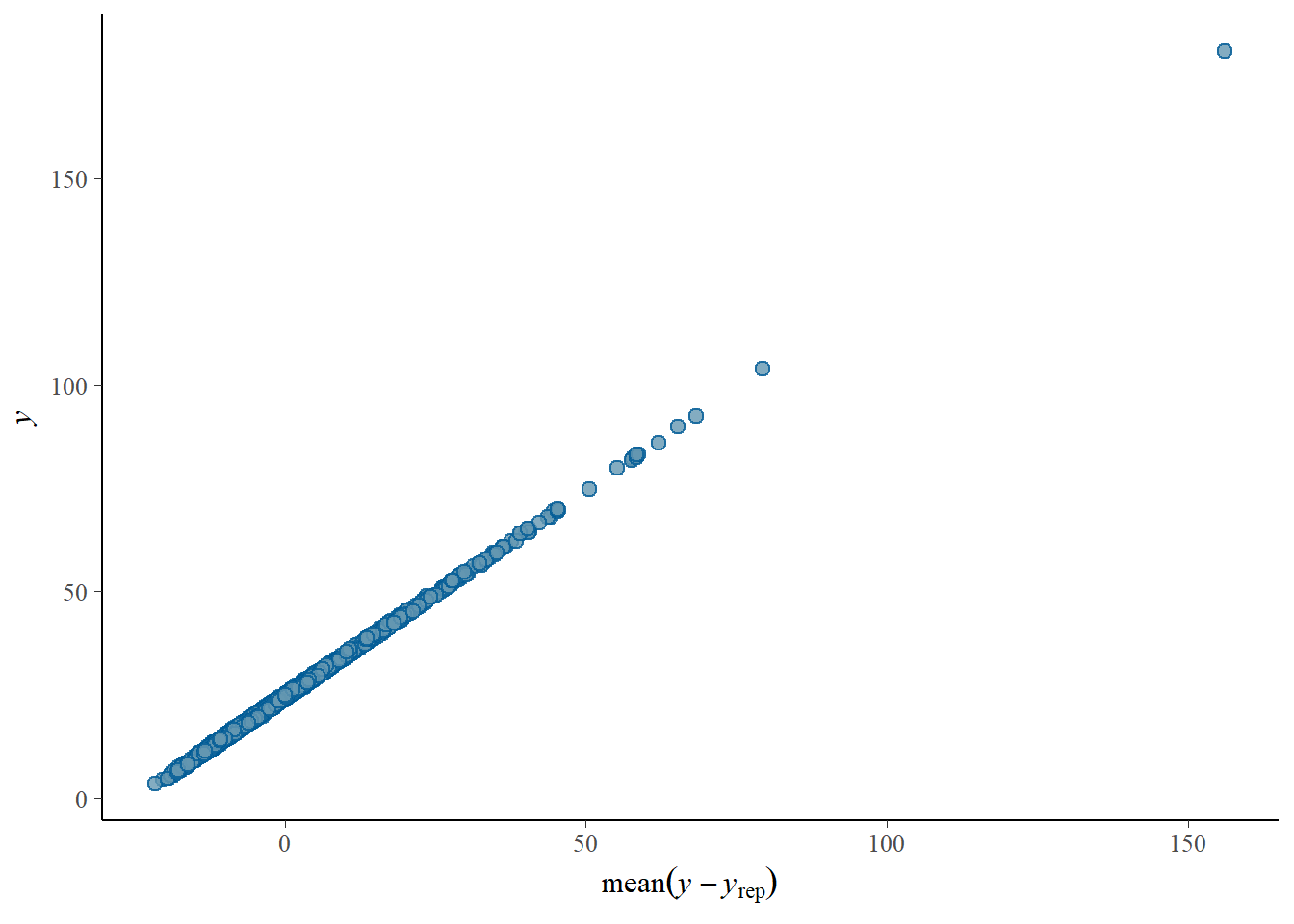
The posterior distribution fits well the predicted data, but the residual error plot points to strong correlation between values and residual.

Model 1 - Varying slopes and intercepts

We will need to add some extra priors now.

• expressibility: A 1 SD change in expressibility is unlikely to change arm moment by more than ×1.4 in either direction (normal(0, 0.35)). We expect a modest effect if any.

• familiarity and BFI: A 1 SD change is unlikely to change arm moment by more than ×1.3 in either direction (normal(0, 0.25)). We expect these to have small effects if any.

• Modality: Switching modality could plausibly up to roughly double or halve arm moment (normal(0, 0.4), exp(±0.8) ≈ ×2.2 at 2 SD). We allow a larger range here than for continuous predictors, reflecting genuine uncertainty about modality effects.

• sigma: Within a given combination of participant, concept and correction phase, individual observations are unlikely to deviate by more than ×1.5 above or below their cell mean (normal(0, 0.4)). Residual spread is expected to be modest.

• sd of pcn_ID, concept and SessionID: Participants, concepts and dyads differ from the population mean by at most ~40% in either direction (normal(0, 0.35), exp(±0.35) ≈ ×1.4). Allows meaningful individual differences without permitting implausibly huge variation.

• sd of trial number: Trial-to-trial drift in arm moment is expected to be very small — most likely within ±16% of the mean (normal(0, 0.15), exp(±0.15)), reflecting a minor practice or fatigue trend rather than a large systematic shift.

Now we do prior predictive check

priors_h1m1_torq_cum <- c(
  set_prior("normal(11, 2)", class = "Intercept"),
  set_prior("normal(0,0.25)", class = "b", coef = "BFI_extra"),
  set_prior("normal(0,0.4)", class = "b", coef = "correction2M1"),
  set_prior("normal(0,0.4)", class = "b", coef = "correction3M2"),
  set_prior("normal(0,0.35)", class = "b", coef = "expressibility_z"),
  set_prior("normal(0,0.25)", class = "b", coef = "Familiarity"),
  set_prior("normal(0,0.4)", class = "b", coef = "modality1"),
  set_prior("normal(0, 0.15)", class = "b", coef = "TrialNumber_c"),
  set_prior("normal(0, 0.4)", class = "sigma"),
  set_prior("normal(0, 0.35)", class = "sd", group = "pcn_ID"),
  set_prior("normal(0, 0.35)", class = "sd", group = "concept"),
  set_prior("normal(0, 0.35)", class = "sd", group = "SessionID"),
  set_prior("lkj(4)", class = "cor")              # regularize, global
)

if (file.exists(here(models, "m_prior_check.rds"))){
  
  m_prior_check <- readRDS(here(models, "m_prior_check.rds"))
  
} else {
  m_prior_check <- brm(
    arm_moment_sum_change_integral ~ 1 + correction + modality + BFI_extra + Familiarity + expressibility_z + TrialNumber_c +  (1 + correction | pcn_ID)  + (1 | SessionID) + (1 + correction | concept),
    data = df_ges,
    family = lognormal(),
    prior = priors_h1m1_torq_cum,
    sample_prior = "only",
    iter = 2000,
    cores = 4
  )
  
  # Save both as objects
  saveRDS(m_prior_check, here(models, "m_prior_check.rds"))

}

# Check prior distribution
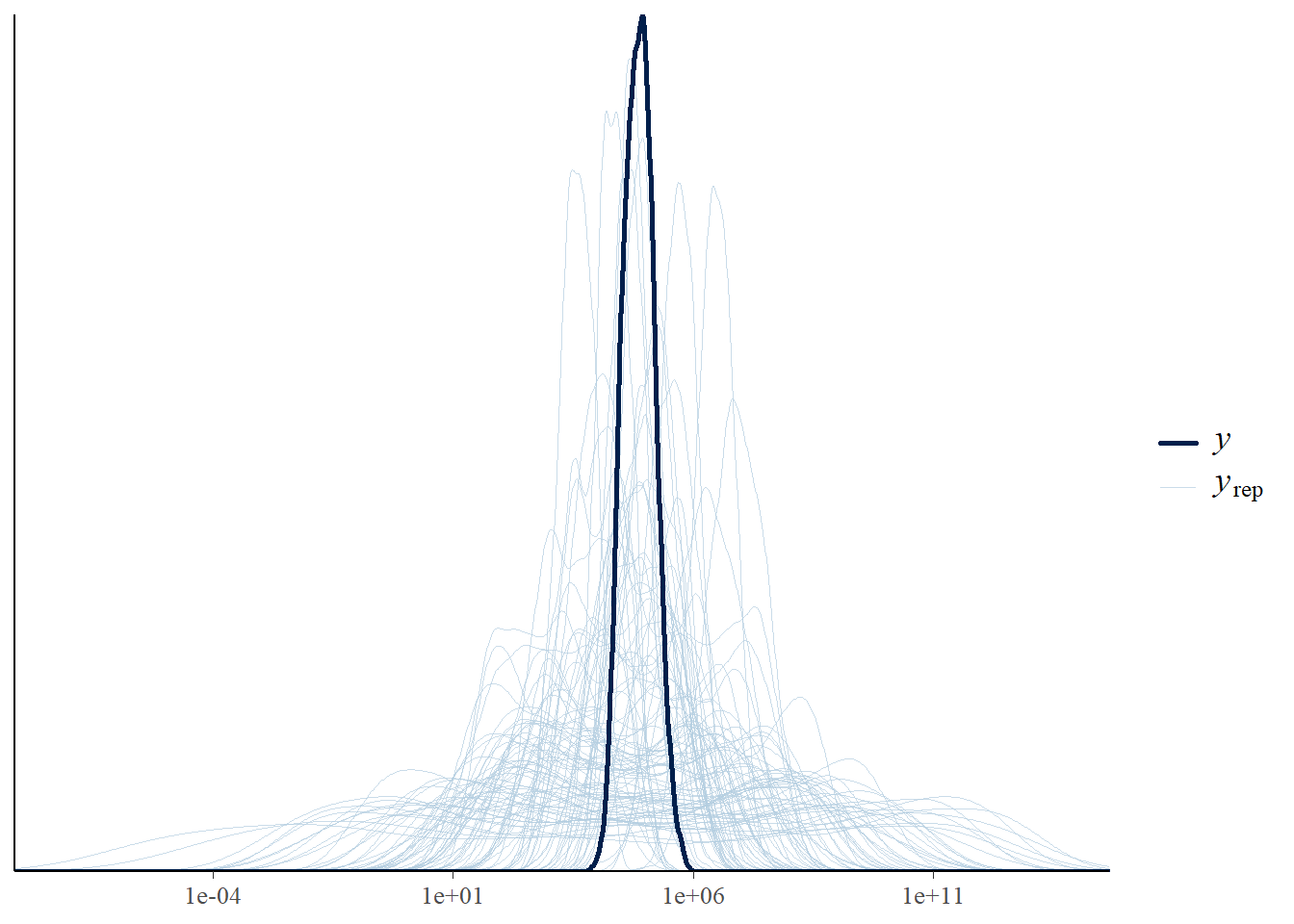
pp_check(m_prior_check, type = "dens_overlay", ndraws = 100) +
  scale_x_log10()

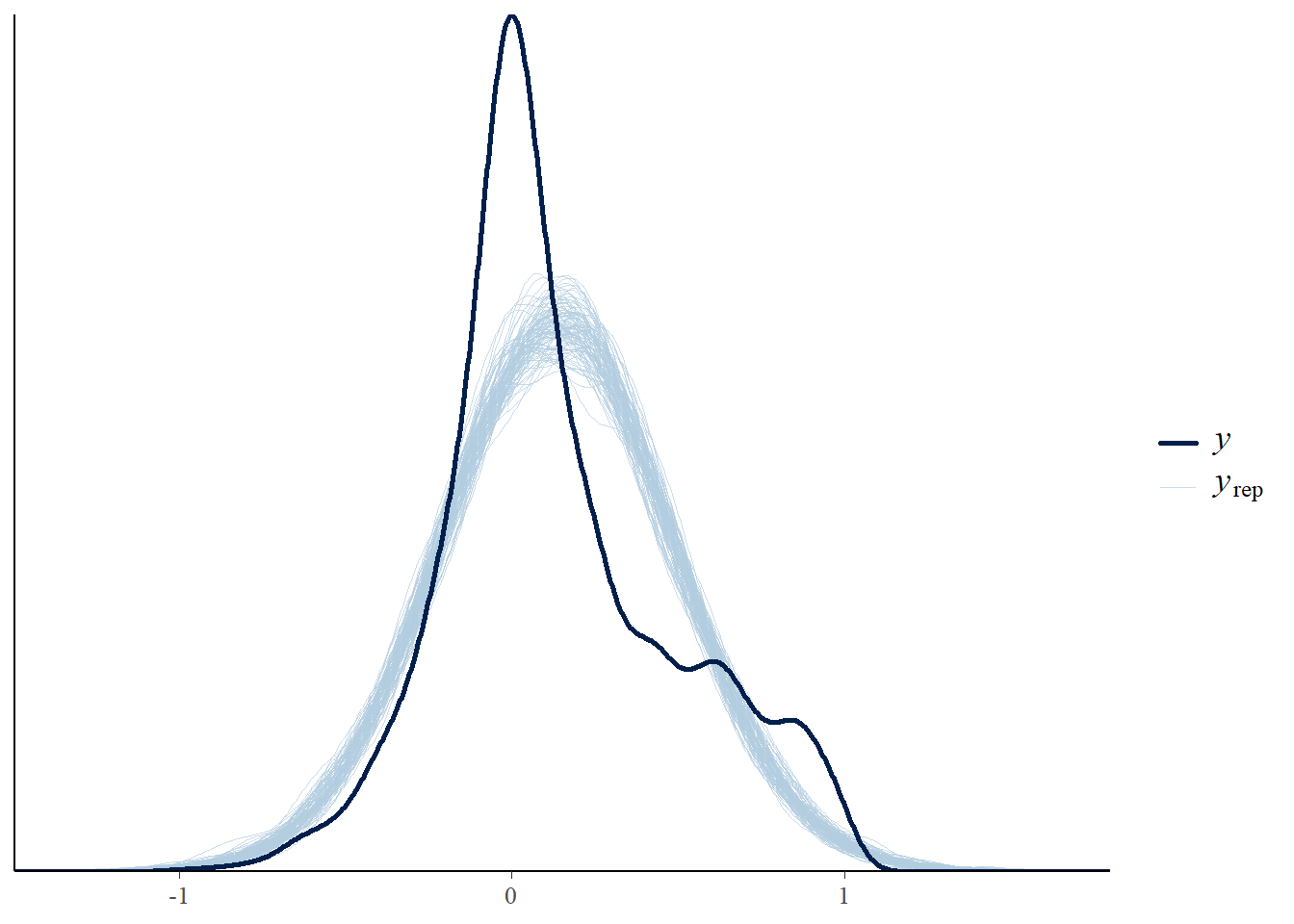
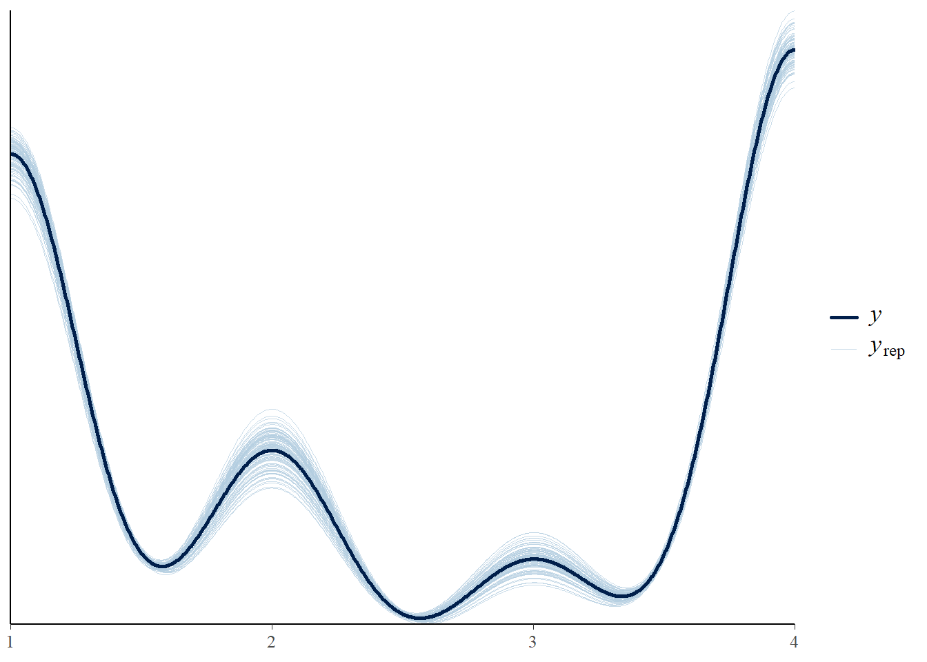
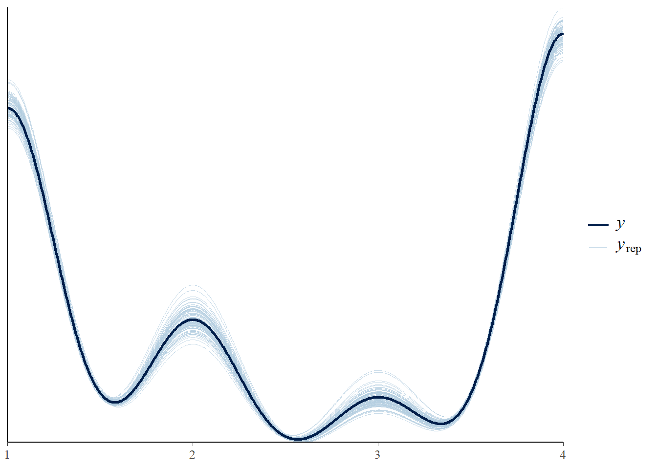
This looks okay. Given that we want to use weakly informative priors, we will not further limit them to avoid the few extreme predictions. Our data should be strong enough to guide the posterior from extremely implausible values with no issues.

if (file.exists(here(models, "h1.m1_torq_cum.rds"))){
  
  h1.m1_torq_cum <- readRDS(here(models, "h1.m1_torq_cum.rds"))
  h1.m1_torq_cum_R2 <- readRDS(here(models, "h1.m1_torq_cum_R2.rds"))
  
} else {
  
  
  h1.m1_torq_cum <- brm(arm_moment_sum_change_integral ~ 1 + correction + modality + BFI_extra + Familiarity + expressibility_z + TrialNumber_c +  (1 + correction | pcn_ID)  + (1 | SessionID) + (1 + correction | concept), 
                  data = df_ges,
                  family = lognormal(),
                  prior = priors_h1m1_torq_cum,
                  iter = 6000, # increase iterations to accomodate more parameters in the model
                  cores = 4,
                  seed = 0209)
  
  # Add criterions for later diagnostics
  h1.m1_torq_cum <- add_criterion(h1.m1_torq_cum, criterion = c("loo", "waic"))
  
  # Calculate also variance explained (R^2)
  h1.m1_torq_cum_R2 <- bayes_R2(h1.m1_torq_cum)
  
  # Save both as objects
  saveRDS(h1.m1_torq_cum, here(models, "h1.m1_torq_cum.rds"))
  saveRDS(h1.m1_torq_cum_R2, here(models, "h1.m1_torq_cum_R2.rds"))

}

# Summary
summary(h1.m1_torq_cum)

 Family: lognormal 
  Links: mu = identity 
Formula: arm_moment_sum_change_integral ~ 1 + correction + modality + BFI_extra + Familiarity + expressibility_z + TrialNumber_c + (1 + correction | pcn_ID) + (1 | SessionID) + (1 + correction | concept) 
   Data: df_ges (Number of observations: 2495) 
  Draws: 4 chains, each with iter = 6000; warmup = 3000; thin = 1;
         total post-warmup draws = 12000

Multilevel Hyperparameters:
~concept (Number of levels: 84) 
                                 Estimate Est.Error l-95% CI u-95% CI Rhat
sd(Intercept)                        0.37      0.03     0.31     0.44 1.00
sd(correction2M1)                    0.03      0.02     0.00     0.09 1.00
sd(correction3M2)                    0.06      0.04     0.00     0.15 1.00
cor(Intercept,correction2M1)        -0.14      0.30    -0.68     0.49 1.00
cor(Intercept,correction3M2)        -0.20      0.28    -0.69     0.40 1.00
cor(correction2M1,correction3M2)     0.01      0.32    -0.58     0.60 1.00
                                 Bulk_ESS Tail_ESS
sd(Intercept)                        1807     3786
sd(correction2M1)                    4435     4490
sd(correction3M2)                    3629     4912
cor(Intercept,correction2M1)        13910     8648
cor(Intercept,correction3M2)        11604     8342
cor(correction2M1,correction3M2)     9057     9098

~pcn_ID (Number of levels: 122) 
                                 Estimate Est.Error l-95% CI u-95% CI Rhat
sd(Intercept)                        0.26      0.03     0.20     0.32 1.00
sd(correction2M1)                    0.13      0.04     0.04     0.20 1.00
sd(correction3M2)                    0.04      0.03     0.00     0.12 1.00
cor(Intercept,correction2M1)         0.19      0.22    -0.27     0.58 1.00
cor(Intercept,correction3M2)        -0.04      0.31    -0.62     0.55 1.00
cor(correction2M1,correction3M2)     0.04      0.31    -0.55     0.63 1.00
                                 Bulk_ESS Tail_ESS
sd(Intercept)                        2464     4203
sd(correction2M1)                    1988     1493
sd(correction3M2)                    4992     6193
cor(Intercept,correction2M1)         4177     5266
cor(Intercept,correction3M2)        15038     8729
cor(correction2M1,correction3M2)    13558     8600

~SessionID (Number of levels: 61) 
              Estimate Est.Error l-95% CI u-95% CI Rhat Bulk_ESS Tail_ESS
sd(Intercept)     0.31      0.04     0.23     0.40 1.00     2583     4001

Regression Coefficients:
                 Estimate Est.Error l-95% CI u-95% CI Rhat Bulk_ESS Tail_ESS
Intercept           11.33      0.06    11.21    11.45 1.00     1760     3379
correction2M1        0.19      0.03     0.13     0.24 1.00    10714     9411
correction3M2        0.15      0.03     0.08     0.21 1.00    12165     8948
modality1            0.06      0.02     0.01     0.10 1.00    15525     9305
BFI_extra            0.02      0.03    -0.04     0.08 1.00     4360     7089
Familiarity         -0.02      0.04    -0.10     0.06 1.00     3780     5818
expressibility_z    -0.10      0.03    -0.17    -0.04 1.00     1947     3563
TrialNumber_c        0.00      0.00     0.00     0.00 1.00    14255    11003

Further Distributional Parameters:
      Estimate Est.Error l-95% CI u-95% CI Rhat Bulk_ESS Tail_ESS
sigma     0.49      0.01     0.48     0.51 1.00     9766     8384

Draws were sampled using sample(hmc). For each parameter, Bulk_ESS
and Tail_ESS are effective sample size measures, and Rhat is the potential
scale reduction factor on split chains (at convergence, Rhat = 1).

Model 2 - Maximizing random structure

if (file.exists(here(models, "h1.m2_torq_cum.rds"))){
  
  h1.m2_torq_cum <- readRDS(here(models, "h1.m2_torq_cum.rds"))
  h1.m2_torq_cum_R2 <- readRDS(here(models, "h1.m2_torq_cum_R2.rds"))
  
} else {
  
  
  h1.m2_torq_cum <- brm(arm_moment_sum_change_integral ~ 1 + correction + modality + BFI_extra + Familiarity + expressibility_z + TrialNumber_c + (1 + correction + modality + expressibility_z | pcn_ID)  + (1 + Familiarity + BFI_extra | SessionID) + (1 + correction + modality | concept), 
                  data = df_ges,
                  family = lognormal(),
                  prior = priors_h1m1_torq_cum,
                  iter = 10000, # increase iterations to accomodate more parameters in the model
                  warmup = 4000,
                  cores = 4,
                  seed = 0209, 
                  adapt_delta = 0.99)
  
  # Add criterions for later diagnostics
  h1.m2_torq_cum <- add_criterion(h1.m2_torq_cum, criterion = c("loo", "waic"))

  
  # Calculate also variance explained (R^2)
  h1.m2_torq_cum_R2 <- bayes_R2(h1.m2_torq_cum)
  
  # Save both as objects
  saveRDS(h1.m2_torq_cum, here(models, "h1.m2_torq_cum.rds"))
  saveRDS(h1.m2_torq_cum_R2, here(models, "h1.m2_torq_cum_R2.rds"))

}

# Summary
summary(h1.m2_torq_cum)

 Family: lognormal 
  Links: mu = identity 
Formula: arm_moment_sum_change_integral ~ 1 + correction + modality + BFI_extra + Familiarity + expressibility_z + TrialNumber_c + (1 + correction + modality + expressibility_z | pcn_ID) + (1 + Familiarity + BFI_extra | SessionID) + (1 + correction + modality | concept) 
   Data: df_ges (Number of observations: 2495) 
  Draws: 4 chains, each with iter = 10000; warmup = 4000; thin = 1;
         total post-warmup draws = 24000

Multilevel Hyperparameters:
~concept (Number of levels: 84) 
                                 Estimate Est.Error l-95% CI u-95% CI Rhat
sd(Intercept)                        0.37      0.03     0.31     0.43 1.00
sd(correction2M1)                    0.04      0.03     0.00     0.09 1.00
sd(correction3M2)                    0.06      0.04     0.00     0.15 1.00
sd(modality1)                        0.16      0.03     0.10     0.23 1.00
cor(Intercept,correction2M1)        -0.13      0.28    -0.64     0.45 1.00
cor(Intercept,correction3M2)        -0.22      0.27    -0.68     0.37 1.00
cor(correction2M1,correction3M2)     0.01      0.30    -0.56     0.59 1.00
cor(Intercept,modality1)            -0.06      0.16    -0.37     0.25 1.00
cor(correction2M1,modality1)         0.13      0.30    -0.47     0.66 1.00
cor(correction3M2,modality1)         0.11      0.28    -0.47     0.62 1.00
                                 Bulk_ESS Tail_ESS
sd(Intercept)                        4533     9764
sd(correction2M1)                    7633    11073
sd(correction3M2)                    6049     9295
sd(modality1)                        8550     9983
cor(Intercept,correction2M1)        31529    18422
cor(Intercept,correction3M2)        26723    16573
cor(correction2M1,correction3M2)    20240    18575
cor(Intercept,modality1)            21496    17037
cor(correction2M1,modality1)         3872     7537
cor(correction3M2,modality1)         4661     8479

~pcn_ID (Number of levels: 122) 
                                    Estimate Est.Error l-95% CI u-95% CI Rhat
sd(Intercept)                           0.23      0.04     0.16     0.31 1.00
sd(correction2M1)                       0.13      0.04     0.04     0.20 1.00
sd(correction3M2)                       0.04      0.03     0.00     0.12 1.00
sd(modality1)                           0.24      0.03     0.18     0.30 1.00
sd(expressibility_z)                    0.05      0.02     0.01     0.09 1.00
cor(Intercept,correction2M1)            0.14      0.22    -0.32     0.53 1.00
cor(Intercept,correction3M2)           -0.04      0.28    -0.56     0.51 1.00
cor(correction2M1,correction3M2)        0.03      0.28    -0.51     0.57 1.00
cor(Intercept,modality1)               -0.17      0.17    -0.48     0.17 1.00
cor(correction2M1,modality1)            0.01      0.20    -0.38     0.40 1.00
cor(correction3M2,modality1)           -0.06      0.27    -0.57     0.48 1.00
cor(Intercept,expressibility_z)        -0.29      0.24    -0.71     0.25 1.00
cor(correction2M1,expressibility_z)    -0.03      0.26    -0.53     0.46 1.00
cor(correction3M2,expressibility_z)     0.03      0.28    -0.53     0.56 1.00
cor(modality1,expressibility_z)         0.23      0.22    -0.25     0.62 1.00
                                    Bulk_ESS Tail_ESS
sd(Intercept)                           3713     7778
sd(correction2M1)                       5180     4714
sd(correction3M2)                       8983    10421
sd(modality1)                          12695    16634
sd(expressibility_z)                    4504     4385
cor(Intercept,correction2M1)            9489    13890
cor(Intercept,correction3M2)           34326    17449
cor(correction2M1,correction3M2)       32046    17849
cor(Intercept,modality1)                5632    10541
cor(correction2M1,modality1)            4235     7962
cor(correction3M2,modality1)            2063     5244
cor(Intercept,expressibility_z)        10068    13355
cor(correction2M1,expressibility_z)    14248    17807
cor(correction3M2,expressibility_z)     9626    15790
cor(modality1,expressibility_z)        17859    15384

~SessionID (Number of levels: 61) 
                           Estimate Est.Error l-95% CI u-95% CI Rhat Bulk_ESS
sd(Intercept)                  0.30      0.05     0.21     0.40 1.00     6268
sd(Familiarity)                0.09      0.06     0.00     0.22 1.00     3232
sd(BFI_extra)                  0.10      0.06     0.01     0.22 1.00     2597
cor(Intercept,Familiarity)    -0.13      0.28    -0.65     0.45 1.00    17989
cor(Intercept,BFI_extra)       0.19      0.26    -0.38     0.64 1.00    12451
cor(Familiarity,BFI_extra)    -0.07      0.31    -0.64     0.55 1.00     8605
                           Tail_ESS
sd(Intercept)                  7681
sd(Familiarity)                9037
sd(BFI_extra)                  5708
cor(Intercept,Familiarity)    17806
cor(Intercept,BFI_extra)      12829
cor(Familiarity,BFI_extra)    12946

Regression Coefficients:
                 Estimate Est.Error l-95% CI u-95% CI Rhat Bulk_ESS Tail_ESS
Intercept           11.33      0.06    11.20    11.45 1.00     4643     8372
correction2M1        0.19      0.03     0.14     0.24 1.00    24468    18830
correction3M2        0.14      0.03     0.08     0.20 1.00    29451    18662
modality1            0.05      0.04    -0.02     0.13 1.00    16206    18582
BFI_extra            0.03      0.03    -0.04     0.10 1.00    12855    14952
Familiarity         -0.02      0.04    -0.11     0.07 1.00    12926    14277
expressibility_z    -0.08      0.04    -0.16    -0.01 1.00     4656     8637
TrialNumber_c        0.00      0.00    -0.00     0.00 1.00    22848    19888

Further Distributional Parameters:
      Estimate Est.Error l-95% CI u-95% CI Rhat Bulk_ESS Tail_ESS
sigma     0.47      0.01     0.45     0.48 1.00    16950    17703

Draws were sampled using sample(hmc). For each parameter, Bulk_ESS
and Tail_ESS are effective sample size measures, and Rhat is the potential
scale reduction factor on split chains (at convergence, Rhat = 1).

Model 3 - Simplification (no correlations)

priors_h1m3_torq_cum <- c(
  set_prior("normal(11, 2)", class = "Intercept"),
  set_prior("normal(0,0.25)", class = "b", coef = "BFI_extra"),
  set_prior("normal(0,0.4)", class = "b", coef = "correction2M1"),
  set_prior("normal(0,0.4)", class = "b", coef = "correction3M2"),
  set_prior("normal(0,0.35)", class = "b", coef = "expressibility_z"),
  set_prior("normal(0,0.25)", class = "b", coef = "Familiarity"),
  set_prior("normal(0,0.4)", class = "b", coef = "modality1"),
  set_prior("normal(0, 0.15)", class = "b", coef = "TrialNumber_c"),
  set_prior("normal(0, 0.4)", class = "sigma"),
  set_prior("normal(0, 0.35)", class = "sd", group = "pcn_ID"),
  set_prior("normal(0, 0.35)", class = "sd", group = "concept"),
  set_prior("normal(0, 0.35)", class = "sd", group = "SessionID")
)

if (file.exists(here(models, "h1.m3_torq_cum.rds"))){
  
  h1.m3_torq_cum <- readRDS(here(models, "h1.m3_torq_cum.rds"))
  h1.m3_torq_cum_R2 <- readRDS(here(models, "h1.m3_torq_cum_R2.rds"))
  
} else {
  
  
  h1.m3_torq_cum <- brm(arm_moment_sum_change_integral ~ 
  1 + correction + modality + BFI_extra + Familiarity + 
  expressibility_z + TrialNumber_c +
  (1 + expressibility_z + correction + modality || pcn_ID) +       
  (1 + Familiarity + BFI_extra || SessionID) +              
  (1 + correction + modality || concept),         
                  data = df_ges,
                  family = lognormal(),
                  prior = priors_h1m3_torq_cum,
                  iter = 10000, # increase iterations to accomodate more parameters in the model
                  warmup = 4000,
                  cores = 4,
                  seed = 0209, 
                  control = list(
                    adapt_delta  = 0.99,
                    max_treedepth = 15)) 
  
  # Add criterions for later diagnostics
  h1.m3_torq_cum <- add_criterion(h1.m3_torq_cum, criterion = c("loo", "waic")) # Waic warning
  
  # Calculate also variance explained (R^2)
  h1.m3_torq_cum_R2 <- bayes_R2(h1.m3_torq_cum)
  
  # Save both as objects
  saveRDS(h1.m3_torq_cum, here(models, "h1.m3_torq_cum.rds"))
  saveRDS(h1.m3_torq_cum_R2, here(models, "h1.m3_torq_cum_R2.rds"))

}

# Summary
summary(h1.m3_torq_cum)

 Family: lognormal 
  Links: mu = identity 
Formula: arm_moment_sum_change_integral ~ 1 + correction + modality + BFI_extra + Familiarity + expressibility_z + TrialNumber_c + (1 + expressibility_z + correction + modality || pcn_ID) + (1 + Familiarity + BFI_extra || SessionID) + (1 + correction + modality || concept) 
   Data: df_ges (Number of observations: 2495) 
  Draws: 4 chains, each with iter = 10000; warmup = 4000; thin = 1;
         total post-warmup draws = 24000

Multilevel Hyperparameters:
~concept (Number of levels: 84) 
                  Estimate Est.Error l-95% CI u-95% CI Rhat Bulk_ESS Tail_ESS
sd(Intercept)         0.37      0.03     0.31     0.44 1.00     3673     8093
sd(correction2M1)     0.03      0.02     0.00     0.09 1.00     7995     9954
sd(correction3M2)     0.06      0.04     0.00     0.15 1.00     5607     9009
sd(modality1)         0.16      0.03     0.10     0.23 1.00     7814     9547

~pcn_ID (Number of levels: 122) 
                     Estimate Est.Error l-95% CI u-95% CI Rhat Bulk_ESS
sd(Intercept)            0.22      0.03     0.16     0.29 1.00     4102
sd(expressibility_z)     0.04      0.02     0.00     0.08 1.00     3993
sd(correction2M1)        0.13      0.04     0.05     0.20 1.00     4876
sd(correction3M2)        0.04      0.03     0.00     0.12 1.00     9100
sd(modality1)            0.24      0.03     0.18     0.30 1.00    10465
                     Tail_ESS
sd(Intercept)            8698
sd(expressibility_z)     6981
sd(correction2M1)        4106
sd(correction3M2)        9979
sd(modality1)           15011

~SessionID (Number of levels: 61) 
                Estimate Est.Error l-95% CI u-95% CI Rhat Bulk_ESS Tail_ESS
sd(Intercept)       0.31      0.04     0.22     0.40 1.00     6748     8327
sd(Familiarity)     0.09      0.06     0.00     0.21 1.00     3608     8047
sd(BFI_extra)       0.10      0.06     0.01     0.21 1.00     2622     6247

Regression Coefficients:
                 Estimate Est.Error l-95% CI u-95% CI Rhat Bulk_ESS Tail_ESS
Intercept           11.33      0.06    11.20    11.45 1.00     4509     8834
correction2M1        0.19      0.03     0.14     0.24 1.00    20269    18728
correction3M2        0.14      0.03     0.08     0.20 1.00    24087    18930
modality1            0.05      0.04    -0.02     0.13 1.00    12964    15624
BFI_extra            0.03      0.03    -0.04     0.10 1.00    11651    14977
Familiarity         -0.02      0.04    -0.10     0.07 1.00    11549    14627
expressibility_z    -0.08      0.04    -0.16    -0.01 1.00     3883     7348
TrialNumber_c        0.00      0.00    -0.00     0.00 1.00    16327    18447

Further Distributional Parameters:
      Estimate Est.Error l-95% CI u-95% CI Rhat Bulk_ESS Tail_ESS
sigma     0.47      0.01     0.45     0.48 1.00    16076    15832

Draws were sampled using sample(hmc). For each parameter, Bulk_ESS
and Tail_ESS are effective sample size measures, and Rhat is the potential
scale reduction factor on split chains (at convergence, Rhat = 1).

Before running interactions, let’s look at the 4 models so far

Diagnostics

We now have several models that we can test for predictive performance.

model_list <- list(m0 = h1.m0_torq_cum, 
                   m1 = h1.m1_torq_cum, 
                   m2 = h1.m2_torq_cum, 
                   m3 = h1.m3_torq_cum 
                   )

Rhat

Rhat tells us whether the model’s Markov chains have converged—values close to 1 mean the model has likely converged well.

# Extract R-hat values for each model
rhat_list <- lapply(model_list, function(model) {
  rhat_values <- rhat(model)
  data.frame(model = deparse(substitute(model)), 
             max_rhat = max(rhat_values), 
             min_rhat = min(rhat_values))
})

# Combine and inspect
do.call(rbind, rhat_list)

    model max_rhat  min_rhat
m0 X[[i]] 1.001537 0.9999976
m1 X[[i]] 1.002489 0.9997962
m2 X[[i]] 1.001467 0.9998969
m3 X[[i]] 1.001689 0.9998770

They all converge well (note that m1 has 4k iterations)

ESS

Effective sample size tells how many independent samples the model has effectively drawn from the PD. Low ESS suggests autocorrelation (i.e., sample explores one part of posterior), while high ESS means good mix

# Extract n_eff values for each model
neff_ratio_list <- lapply(model_list, function(model) {
  neff_values <- neff_ratio(model)              # Here we calculate ratio (not the raw number of effective samples)
  data.frame(model = deparse(substitute(model)), 
             min_neff = min(neff_values), 
             max_neff = max(neff_values),
             mean_neff = mean(neff_values))
               
})

# Combine and inspect
do.call(rbind, neff_ratio_list)

    model   min_neff  max_neff mean_neff
m0 X[[i]] 0.53905959 0.8726148 0.7447865
m1 X[[i]] 0.12440670 0.9169455 0.6503774
m2 X[[i]] 0.08595817 0.8972331 0.6965750
m3 X[[i]] 0.10923467 0.8418179 0.6815941

We can see that no correlations helped

LOO

Leave-One-Out (LOO) validation is a technique where, for each iteration, one data point is left out as the test set, and the model is trained on the remaining data points; this process is repeated for each data point, and the model’s overall performance is averaged over all iterations.

l <- loo_compare(h1.m0_torq_cum, h1.m1_torq_cum, h1.m2_torq_cum, h1.m3_torq_cum, criterion = "loo")

print(l, simplify = F)

               elpd_diff se_diff  elpd_loo se_elpd_loo p_loo    se_p_loo
h1.m2_torq_cum      0.0       0.0 -29782.9     51.4       335.5      9.0
h1.m3_torq_cum     -0.6       1.9 -29783.5     51.4       333.6      8.9
h1.m1_torq_cum    -51.0      10.2 -29833.9     51.1       227.3      6.3
h1.m0_torq_cum   -886.1      35.2 -30668.9     52.1         3.8      0.1
               looic    se_looic
h1.m2_torq_cum  59565.8    102.8
h1.m3_torq_cum  59566.9    102.8
h1.m1_torq_cum  59667.8    102.2
h1.m0_torq_cum  61337.9    104.2

Loo evaluates as best the model with maximal random structure, but eff for this model have some low-performing parameters. Given that m3 is in loo tightly behind, we will use m3 for interactions too.

Model 4 - Adding interactions

Possible interactions include:

• CommAtt x Modality - Effort could increase differently across modalities, depending on whether concept is guessed on the first, second or third attempt. E.g., gesture might require more effort on initial attempt, but vocal require more effort in repeated attempt. This is interesting question and it would help disentangle the benfit of multimodality over unimodality (i.e., multimodal trials might be more effortful, but overal have less attempts). However, we already model effect of modality on effort, so maybe this is not top priority.

• CommAtt x Expressibility - Higher expressibility should moderate the effect of repeated attempts, such that the increase in effort with each additional attempt is smaller (or bigger?) for more expressible concepts.This is not a priority for our analysis.

• Modality × Expressibility_z - The influence of expressibility on effort could be modality-specific — perhaps effort increases less with expressibility in the combined modality. For our analysis, this is also not a priority (especially since expressibiliy has already modality encoded)

• Familiarity x CommAtt - More familiar partners may guess faster (fewer attempts) and require less effort, but this effect could diminish over multiple attempts. For our analysis, this is not a priority,

• Big5 × Modality or Big5 × CommAtt - More open/extraverted participants might maintain higher effort over attempts, or adjust more dynamically depending on the communicative channel. While not priority, it is an interesting question if we want to tap more into the inter-individual variability.

if (file.exists(here(models, "h1.m4_torq_cum.rds"))){
  
  h1.m4_torq_cum <- readRDS(here(models, "h1.m4_torq_cum.rds"))
  h1.m4_torq_cum_R2 <- readRDS(here(models, "h1.m4_torq_cum_R2.rds"))
  
} else {
  
  
  h1.m4_torq_cum <- brm(arm_moment_sum_change_integral ~ 
  1 + 
    correction + modality + expressibility_z + BFI_extra + Familiarity + 
    TrialNumber_c +
    correction:modality +           
    correction:expressibility_z +   
    modality:expressibility_z +     
    correction:BFI_extra +          
    correction:Familiarity +        
    (1 + correction + modality + correction:modality || pcn_ID) +
    (1 + Familiarity + BFI_extra || SessionID) +
    (1 + correction + modality || concept),
                  data = df_ges,
                  family = lognormal(),
                  prior = priors_h1m3_torq_cum,
                  iter = 10000, # increase iterations to accomodate more parameters in the model
                  warmup = 4000,
                  cores = 4,
                  seed = 0209, 
                  adapt_delta = 0.99)
  
  # Add criterions for later diagnostics
  h1.m4_torq_cum <- add_criterion(h1.m4_torq_cum, criterion = c("loo", "waic"))
  
  # Calculate also variance explained (R^2)
  h1.m4_torq_cum_R2 <- bayes_R2(h1.m4_torq_cum)
  
  # Save both as objects
  saveRDS(h1.m4_torq_cum, here(models, "h1.m4_torq_cum.rds"))
  saveRDS(h1.m4_torq_cum_R2, here(models, "h1.m4_torq_cum_R2.rds"))

}

# Summary
summary(h1.m4_torq_cum)

 Family: lognormal 
  Links: mu = identity 
Formula: arm_moment_sum_change_integral ~ 1 + correction + modality + expressibility_z + BFI_extra + Familiarity + TrialNumber_c + correction:modality + correction:expressibility_z + modality:expressibility_z + correction:BFI_extra + correction:Familiarity + (1 + correction + modality + correction:modality || pcn_ID) + (1 + Familiarity + BFI_extra || SessionID) + (1 + correction + modality || concept) 
   Data: df_ges (Number of observations: 2495) 
  Draws: 4 chains, each with iter = 10000; warmup = 4000; thin = 1;
         total post-warmup draws = 24000

Multilevel Hyperparameters:
~concept (Number of levels: 84) 
                  Estimate Est.Error l-95% CI u-95% CI Rhat Bulk_ESS Tail_ESS
sd(Intercept)         0.37      0.03     0.31     0.44 1.00     4646     9597
sd(correction2M1)     0.03      0.02     0.00     0.09 1.00     8491    10992
sd(correction3M2)     0.06      0.04     0.00     0.15 1.00     6438    10005
sd(modality1)         0.16      0.03     0.10     0.23 1.00     8251    10265

~pcn_ID (Number of levels: 122) 
                            Estimate Est.Error l-95% CI u-95% CI Rhat Bulk_ESS
sd(Intercept)                   0.22      0.03     0.16     0.29 1.00     5164
sd(correction2M1)               0.14      0.03     0.06     0.20 1.00     6133
sd(correction3M2)               0.04      0.03     0.00     0.12 1.00     9916
sd(modality1)                   0.24      0.03     0.18     0.30 1.00    11038
sd(correction2M1:modality1)     0.07      0.05     0.00     0.18 1.00     8122
sd(correction3M2:modality1)     0.09      0.06     0.00     0.24 1.00     8404
                            Tail_ESS
sd(Intercept)                   9067
sd(correction2M1)               6177
sd(correction3M2)              12028
sd(modality1)                  16653
sd(correction2M1:modality1)     9767
sd(correction3M2:modality1)    10586

~SessionID (Number of levels: 61) 
                Estimate Est.Error l-95% CI u-95% CI Rhat Bulk_ESS Tail_ESS
sd(Intercept)       0.31      0.04     0.23     0.40 1.00     7637    10687
sd(Familiarity)     0.09      0.06     0.00     0.21 1.00     4057     9009
sd(BFI_extra)       0.10      0.06     0.01     0.21 1.00     2745     6250

Regression Coefficients:
                               Estimate Est.Error l-95% CI u-95% CI Rhat
Intercept                         11.33      0.06    11.20    11.45 1.00
correction2M1                      0.19      0.03     0.14     0.24 1.00
correction3M2                      0.13      0.03     0.07     0.20 1.00
modality1                          0.05      0.04    -0.02     0.13 1.00
expressibility_z                  -0.09      0.04    -0.17    -0.01 1.00
BFI_extra                          0.03      0.03    -0.04     0.10 1.00
Familiarity                       -0.02      0.04    -0.11     0.07 1.00
TrialNumber_c                      0.00      0.00    -0.00     0.00 1.00
correction2M1:modality1           -0.01      0.05    -0.10     0.08 1.00
correction3M2:modality1            0.02      0.06    -0.11     0.14 1.00
correction2M1:expressibility_z     0.01      0.02    -0.03     0.06 1.00
correction3M2:expressibility_z    -0.02      0.03    -0.09     0.04 1.00
modality1:expressibility_z         0.02      0.03    -0.05     0.08 1.00
correction2M1:BFI_extra            0.00      0.03    -0.05     0.05 1.00
correction3M2:BFI_extra           -0.00      0.03    -0.06     0.06 1.00
correction2M1:Familiarity          0.00      0.03    -0.05     0.05 1.00
correction3M2:Familiarity         -0.01      0.03    -0.07     0.06 1.00
                               Bulk_ESS Tail_ESS
Intercept                          4579     9466
correction2M1                     23978    19624
correction3M2                     27752    20182
modality1                         16782    17599
expressibility_z                   4235     7804
BFI_extra                         14894    14543
Familiarity                       12818    15225
TrialNumber_c                     19901    19513
correction2M1:modality1           29648    18560
correction3M2:modality1           29542    19755
correction2M1:expressibility_z    28419    19102
correction3M2:expressibility_z    26083    18618
modality1:expressibility_z        16212    17595
correction2M1:BFI_extra           22918    18498
correction3M2:BFI_extra           29720    18198
correction2M1:Familiarity         22331    18154
correction3M2:Familiarity         29738    18220

Further Distributional Parameters:
      Estimate Est.Error l-95% CI u-95% CI Rhat Bulk_ESS Tail_ESS
sigma     0.47      0.01     0.46     0.49 1.00    19077    17663

Draws were sampled using sample(hmc). For each parameter, Bulk_ESS
and Tail_ESS are effective sample size measures, and Rhat is the potential
scale reduction factor on split chains (at convergence, Rhat = 1).

Diagnostics II

Convergence

model_list_torq_cum <- list(m0 = h1.m0_torq_cum, 
                   m1 = h1.m1_torq_cum, 
                   m2 = h1.m2_torq_cum, 
                   m3 = h1.m3_torq_cum,
                   m4 = h1.m4_torq_cum
                   )

convergence_results_tc <- compare_convergence(model_list_torq_cum)

write.csv(convergence_results_tc,
          here(summaries, "convergence_comparison_torq_cum.csv"),
          row.names = FALSE, fileEncoding = "UTF-8")

This is how the models look like, compared on several diagnostics measures

Table 5.1: Cumulative torque: convergence metrics

model	total_draws	neff_thr_bad	neff_thr_crit	max_rhat	n_rhat_bad	min_neff	mean_neff	n_neff_bad	n_neff_crit	min_bulk_ESS	mean_bulk_ESS	n_bulk_bad	n_bulk_crit	min_tail_ESS	mean_tail_ESS	n_tail_bad	n_tail_crit	converged	score
m0	4000	0.2500	0.1000	1.0015	0	0.5391	0.7448	0	0	3025.386	3436	0	0	2812.074	3046	0	0	TRUE	NA
m1	12000	0.0833	0.0333	1.0025	0	0.1244	0.6504	0	0	1760.378	8252	0	0	3378.540	7433	0	0	TRUE	NA
m2	24000	0.0417	0.0167	1.0015	0	0.0860	0.6966	0	0	4642.708	16111	0	0	8372.469	15545	0	0	TRUE	NA
m3	24000	0.0417	0.0167	1.0017	0	0.1092	0.6816	0	0	3883.227	13480	0	0	7348.046	14816	0	0	TRUE	NA
m4	24000	0.0417	0.0167	1.0015	0	0.1144	0.7173	0	0	4235.420	21035	0	0	7803.603	17129	0	0	TRUE	NA

LOO (Predictability)

And this is comparison for Leave-One-Out criteria, assessing the predictive power

l <- loo_compare(h1.m0_torq_cum, h1.m1_torq_cum, h1.m2_torq_cum, h1.m3_torq_cum, h1.m4_torq_cum, criterion = "loo")

print(l, simplify = F)

               elpd_diff se_diff  elpd_loo se_elpd_loo p_loo    se_p_loo
h1.m2_torq_cum      0.0       0.0 -29782.9     51.4       335.5      9.0
h1.m3_torq_cum     -0.6       1.9 -29783.5     51.4       333.6      8.9
h1.m4_torq_cum    -11.1       3.0 -29794.0     51.4       336.8      9.0
h1.m1_torq_cum    -51.0      10.2 -29833.9     51.1       227.3      6.3
h1.m0_torq_cum   -886.1      35.2 -30668.9     52.1         3.8      0.1
               looic    se_looic
h1.m2_torq_cum  59565.8    102.8
h1.m3_torq_cum  59566.9    102.8
h1.m4_torq_cum  59588.0    102.8
h1.m1_torq_cum  59667.8    102.2
h1.m0_torq_cum  61337.9    104.2

For final report, we will use m3 but because they all converged well, we will report differences where relevant. While m2 has better LOO (predictive power), m3 has better ESS which is more important for healthy model

Let’s also check the model visually. Here to see whether all chains converged well

… the relation between predicted and raw data

… residual error

Report

Full comparison

To see whether models drastically differs in estimates, here is a table summary for all available estimates across all five models

model_list_torq_cum <- list(m0 = h1.m0_torq_cum, 
                   m1 = h1.m1_torq_cum, 
                   m2 = h1.m2_torq_cum, 
                   m3 = h1.m3_torq_cum,
                   m4 = h1.m4_torq_cum
                   )

r2_list_torq_cum <- list(m0 = h1.m0_torq_cum_R2, 
                   m1 = h1.m1_torq_cum_R2, 
                   m2 = h1.m2_torq_cum_R2, 
                   m3 = h1.m3_torq_cum_R2,
                   m4 = h1.m4_torq_cum_R2
                   )

# Parameter table
param_table_torq_cum <- create_parameter_table(model_list_torq_cum, r2_list_torq_cum)
write.csv(param_table_torq_cum,
          here(summaries, "parameter_table_h1_torq_cum.csv"),
          row.names = FALSE, fileEncoding = "UTF-8")

Table 5.2: Cumulative torque: summary for all models

term_type	parameter	m0	m1	m2	m3	m4
model_info	R2	0.026 [0.016, 0.039]	0.5 [0.463, 0.536]	0.537 [0.499, 0.573]	0.533 [0.496, 0.568]	0.53 [0.495, 0.565]
model_info	formula	arm_moment_sum_change_integral ~ 1 + correction	arm_moment_sum_change_integral ~ 1 + correction + modality + BFI_extra + Familiarity + expressibility_z + TrialNumber_c + (1 + correction | pcn_ID) + (1 | SessionID) + (1 + correction | concept)	arm_moment_sum_change_integral ~ 1 + correction + modality + BFI_extra + Familiarity + expressibility_z + TrialNumber_c + (1 + correction + modality + expressibility_z | pcn_ID) + (1 + Familiarity + BFI_extra | SessionID) + (1 + correction + modality | concept)	arm_moment_sum_change_integral ~ 1 + correction + modality + BFI_extra + Familiarity + expressibility_z + TrialNumber_c + (1 + expressibility_z + correction + modality || pcn_ID) + (1 + Familiarity + BFI_extra || SessionID) + (1 + correction + modality || concept)	arm_moment_sum_change_integral ~ 1 + correction + modality + expressibility_z + BFI_extra + Familiarity + TrialNumber_c + correction:modality + correction:expressibility_z + modality:expressibility_z + correction:BFI_extra + correction:Familiarity + (1 + correction + modality + correction:modality || pcn_ID) + (1 + Familiarity + BFI_extra || SessionID) + (1 + correction + modality || concept)
model_info	n_obs	2495	2495	2495	2495	2495
fixed	Intercept	11.27 [11.238, 11.302] *	11.329 [11.206, 11.454] *	11.327 [11.203, 11.454] *	11.326 [11.201, 11.451] *	11.328 [11.202, 11.453] *
fixed	BFI_extra	—	0.018 [-0.04, 0.077]	0.028 [-0.037, 0.096]	0.028 [-0.039, 0.097]	0.027 [-0.039, 0.097]
fixed	Familiarity	—	-0.017 [-0.1, 0.063]	-0.019 [-0.109, 0.068]	-0.017 [-0.104, 0.07]	-0.018 [-0.107, 0.069]
fixed	TrialNumber_c	—	0.001 [0, 0.002] *	0.001 [0, 0.002]	0.001 [0, 0.002]	0.001 [0, 0.002]
fixed	correction2M1	0.2 [0.134, 0.265] *	0.188 [0.134, 0.242] *	0.188 [0.136, 0.24] *	0.187 [0.135, 0.24] *	0.189 [0.135, 0.241] *
fixed	correction2M1:BFI_extra	—	—	—	—	0.001 [-0.049, 0.053]
fixed	correction2M1:Familiarity	—	—	—	—	0.001 [-0.051, 0.052]
fixed	correction2M1:expressibility_z	—	—	—	—	0.014 [-0.034, 0.062]
fixed	correction2M1:modality1	—	—	—	—	-0.011 [-0.103, 0.082]
fixed	correction3M2	0.137 [0.048, 0.228] *	0.145 [0.081, 0.211] *	0.139 [0.075, 0.204] *	0.141 [0.078, 0.204] *	0.134 [0.066, 0.201] *
fixed	correction3M2:BFI_extra	—	—	—	—	-0.003 [-0.063, 0.057]
fixed	correction3M2:Familiarity	—	—	—	—	-0.006 [-0.067, 0.055]
fixed	correction3M2:expressibility_z	—	—	—	—	-0.02 [-0.085, 0.044]
fixed	correction3M2:modality1	—	—	—	—	0.017 [-0.106, 0.141]
fixed	expressibility_z	—	-0.104 [-0.171, -0.036] *	-0.083 [-0.156, -0.01] *	-0.083 [-0.158, -0.009] *	-0.09 [-0.169, -0.011] *
fixed	modality1	—	0.057 [0.015, 0.1] *	0.054 [-0.017, 0.125]	0.054 [-0.017, 0.126]	0.054 [-0.022, 0.13]
fixed	modality1:expressibility_z	—	—	—	—	0.016 [-0.046, 0.077]
random_sd	sd() | residual__	0.72 [0.7, 0.74]	0.491 [0.476, 0.506]	0.468 [0.453, 0.483]	0.468 [0.454, 0.484]	0.47 [0.455, 0.485]
random_sd	sd(BFI_extra) | SessionID	—	—	0.101 [0.006, 0.215]	0.098 [0.006, 0.212]	0.098 [0.006, 0.211]
random_sd	sd(Familiarity) | SessionID	—	—	0.092 [0.005, 0.216]	0.088 [0.005, 0.208]	0.09 [0.005, 0.21]
random_sd	sd(Intercept) | SessionID	—	0.308 [0.227, 0.399]	0.305 [0.214, 0.397]	0.31 [0.223, 0.401]	0.31 [0.225, 0.401]
random_sd	sd(Intercept) | concept	—	0.369 [0.312, 0.439]	0.367 [0.309, 0.434]	0.37 [0.313, 0.438]	0.371 [0.314, 0.437]
random_sd	sd(Intercept) | pcn_ID	—	0.256 [0.201, 0.322]	0.231 [0.161, 0.308]	0.224 [0.159, 0.293]	0.223 [0.159, 0.293]
random_sd	sd(correction2M1) | concept	—	0.033 [0.001, 0.088]	0.035 [0.002, 0.092]	0.032 [0.001, 0.089]	0.033 [0.001, 0.091]
random_sd	sd(correction2M1) | pcn_ID	—	0.127 [0.036, 0.195]	0.127 [0.039, 0.198]	0.132 [0.053, 0.197]	0.139 [0.063, 0.202]
random_sd	sd(correction2M1:modality1) | pcn_ID	—	—	—	—	0.066 [0.003, 0.177]
random_sd	sd(correction3M2) | concept	—	0.061 [0.003, 0.146]	0.065 [0.003, 0.15]	0.06 [0.003, 0.149]	0.059 [0.003, 0.15]
random_sd	sd(correction3M2) | pcn_ID	—	0.043 [0.002, 0.118]	0.043 [0.002, 0.118]	0.043 [0.002, 0.118]	0.045 [0.002, 0.123]
random_sd	sd(correction3M2:modality1) | pcn_ID	—	—	—	—	0.09 [0.004, 0.24]
random_sd	sd(expressibility_z) | pcn_ID	—	—	0.05 [0.005, 0.091]	0.041 [0.002, 0.084]	—
random_sd	sd(modality1) | concept	—	—	0.162 [0.097, 0.228]	0.162 [0.097, 0.227]	0.162 [0.097, 0.226]
random_sd	sd(modality1) | pcn_ID	—	—	0.237 [0.183, 0.297]	0.238 [0.183, 0.296]	0.238 [0.183, 0.296]
random_cor	cor(Familiarity x BFI_extra) | SessionID	—	—	-0.068 [-0.641, 0.553]	—	—
random_cor	cor(Intercept x BFI_extra) | SessionID	—	—	0.190 [-0.377, 0.643]	—	—
random_cor	cor(Intercept x Familiarity) | SessionID	—	—	-0.127 [-0.646, 0.448]	—	—
random_cor	cor(Intercept x correction2M1) | concept	—	-0.141 [-0.681, 0.495]	-0.134 [-0.644, 0.450]	—	—
random_cor	cor(Intercept x correction2M1) | pcn_ID	—	0.192 [-0.266, 0.583]	0.139 [-0.316, 0.532]	—	—
random_cor	cor(Intercept x correction3M2) | concept	—	-0.197 [-0.687, 0.399]	-0.215 [-0.681, 0.368]	—	—
random_cor	cor(Intercept x correction3M2) | pcn_ID	—	-0.044 [-0.618, 0.554]	-0.036 [-0.562, 0.507]	—	—
random_cor	cor(Intercept x expressibility_z) | pcn_ID	—	—	-0.293 [-0.708, 0.250]	—	—
random_cor	cor(Intercept x modality1) | concept	—	—	-0.062 [-0.374, 0.252]	—	—
random_cor	cor(Intercept x modality1) | pcn_ID	—	—	-0.172 [-0.484, 0.170]	—	—
random_cor	cor(correction2M1 x correction3M2) | concept	—	0.007 [-0.584, 0.603]	0.014 [-0.564, 0.586]	—	—
random_cor	cor(correction2M1 x correction3M2) | pcn_ID	—	0.043 [-0.554, 0.628]	0.034 [-0.513, 0.573]	—	—
random_cor	cor(correction2M1 x expressibility_z) | pcn_ID	—	—	-0.033 [-0.529, 0.461]	—	—
random_cor	cor(correction2M1 x modality1) | concept	—	—	0.125 [-0.474, 0.658]	—	—
random_cor	cor(correction2M1 x modality1) | pcn_ID	—	—	0.011 [-0.380, 0.401]	—	—
random_cor	cor(correction3M2 x expressibility_z) | pcn_ID	—	—	0.027 [-0.528, 0.564]	—	—
random_cor	cor(correction3M2 x modality1) | concept	—	—	0.110 [-0.469, 0.621]	—	—
random_cor	cor(correction3M2 x modality1) | pcn_ID	—	—	-0.065 [-0.566, 0.479]	—	—
random_cor	cor(modality1 x expressibility_z) | pcn_ID	—	—	0.228 [-0.253, 0.620]	—	—

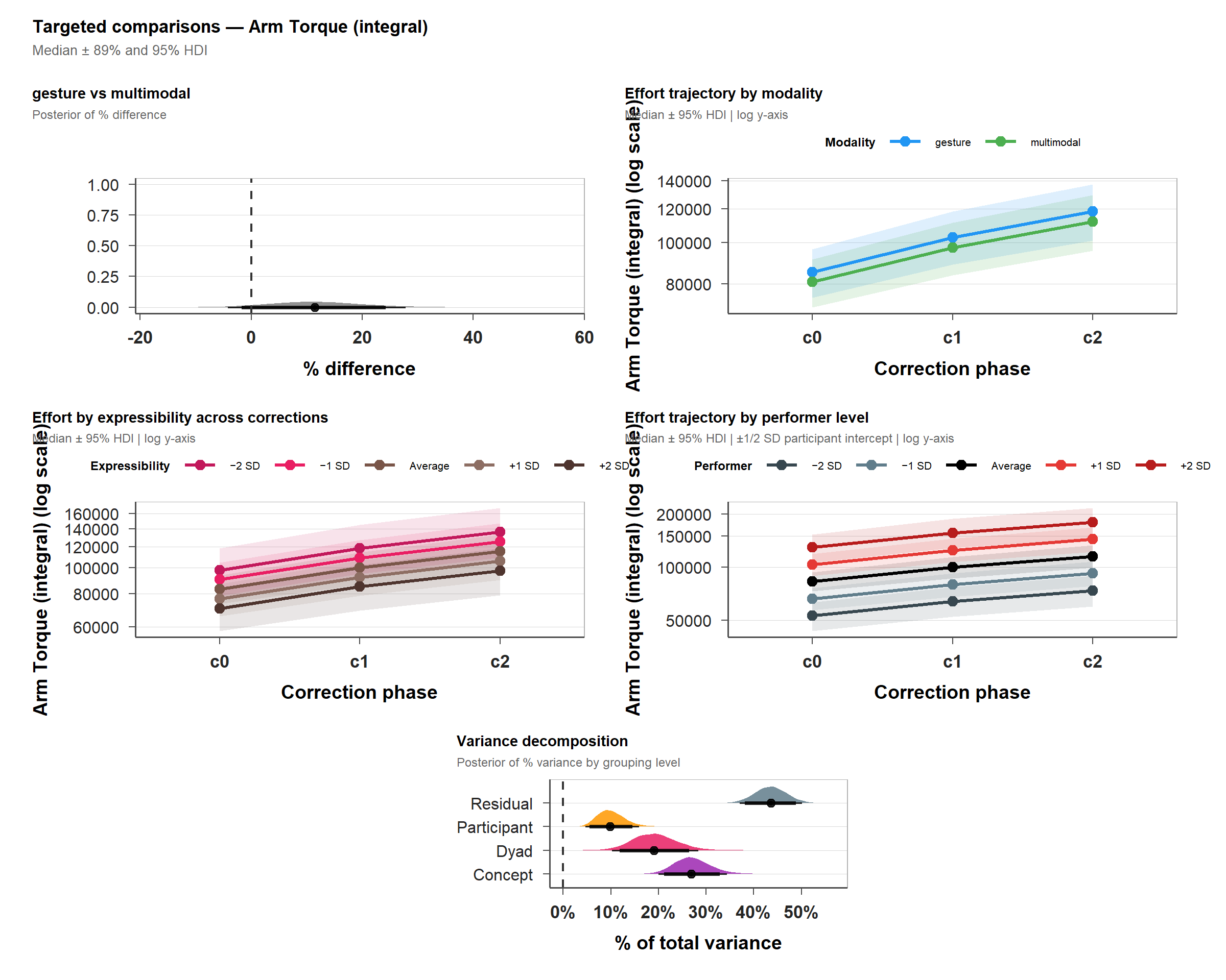
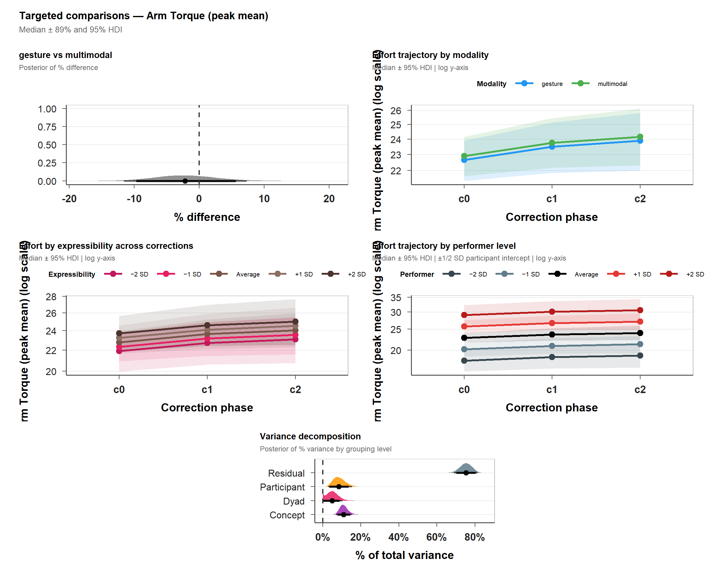
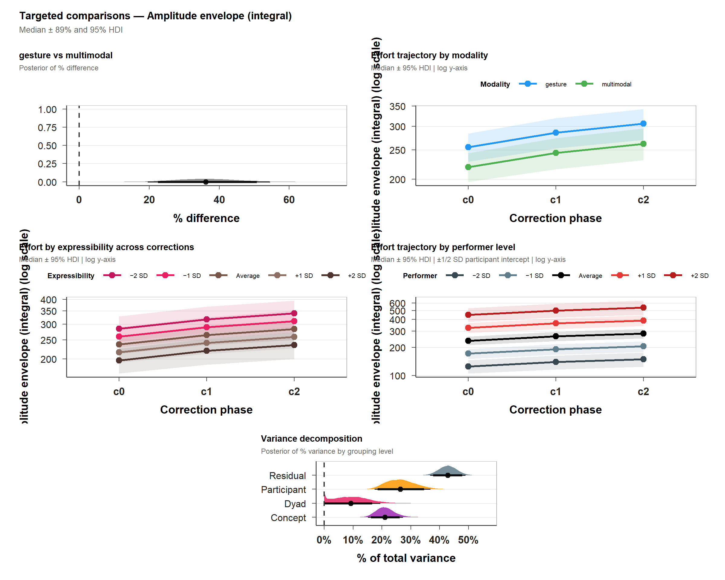
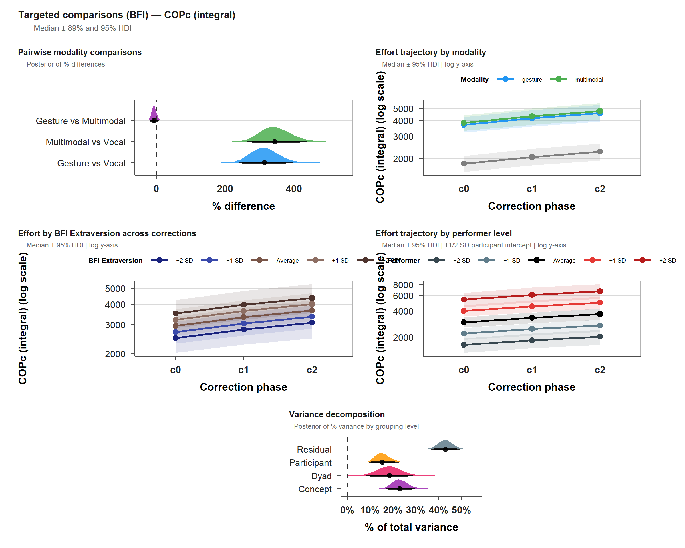
Final model report

And here we report relevant comparisons for selected models, together with visualization

═══════════════════════════════════════════════
  1. MODALITY COMPARISONS (main effect)
═══════════════════════════════════════════════

  gesture vs multimodal (log scale):            0.108 [-0.033, 0.253]
  gesture vs multimodal (%):                    +11.4% [-4.2%, +27.8%]

═══════════════════════════════════════════════
  2. EFFORT BY MODALITY ACROSS CORRECTIONS
═══════════════════════════════════════════════

  Predicted effort (median [95% HDI]):
    gesture c0:                                 85206.586 [74188.452, 96623.067]  *
    gesture c1:                                 102749.959 [88729.755, 118299.865]  *
    gesture c2:                                 118361.520 [101167.785, 137323.236]  *
    multimodal c0:                              80752.309 [70409.855, 91381.874]  *
    multimodal c1:                              97391.051 [83844.287, 111561.992]  *
    multimodal c2:                              112159.273 [95822.006, 129426.105]  *

  Absolute increase per step:
    gesture c0→c1:                            17538.513 [11732.987, 23605.776]  *
    gesture c1→c2:                            15526.795 [8294.980, 23454.572]  *
    multimodal c0→c1:                         16623.550 [11070.174, 22370.704]  *
    multimodal c1→c2:                         14700.756 [7828.757, 22136.671]  *

  gesture vs multimodal at each step (%):
    c0:                                         +5.6% [-2.1%, +13.1%]
    c1:                                         +5.6% [-2.1%, +13.1%]
    c2:                                         +5.6% [-2.1%, +13.1%]

═══════════════════════════════════════════════
  3. EXPRESSIBILITY ACROSS CORRECTIONS (±1 SD and ±2 SD)
═══════════════════════════════════════════════

  Predicted effort (median [95% HDI]):
    Very low (-2SD) c0:                         98066.815 [78482.564, 118460.159]  *
    Very low (-2SD) c1:                         118283.034 [94772.545, 144679.137]  *
    Very low (-2SD) c2:                         136316.293 [109062.570, 167641.847]  *
    Low (-1SD) c0:                              90188.450 [76803.782, 104335.734]  *
    Low (-1SD) c1:                              108792.026 [91732.037, 126880.665]  *
    Low (-1SD) c2:                              125315.255 [104908.244, 146873.570]  *
    Average c0:                                 82927.209 [72978.343, 93734.163]  *
    Average c1:                                 100068.235 [86580.898, 114176.406]  *
    Average c2:                                 115195.284 [99372.080, 133168.032]  *
    High (+1SD) c0:                             76336.434 [65872.372, 87019.630]  *
    High (+1SD) c1:                             92050.728 [78490.549, 106344.223]  *
    High (+1SD) c2:                             106018.233 [89867.249, 123675.463]  *
    Very high (+2SD) c0:                        70256.251 [57785.049, 83767.939]  *
    Very high (+2SD) c1:                        84792.720 [69158.059, 102352.127]  *
    Very high (+2SD) c2:                        97623.764 [78919.899, 118210.440]  *

  Absolute increase per step:
    Low  c0→c1:                               18554.383 [12345.774, 25163.932]  *
    Low  c1→c2:                               16420.578 [8493.357, 24700.571]  *
    Avg  c0→c1:                               17078.553 [11576.982, 23125.354]  *
    Avg  c1→c2:                               15108.555 [7981.825, 22695.374]  *
    High c0→c1:                               15705.110 [10407.746, 21312.299]  *
    High c1→c2:                               13887.210 [7272.729, 20955.617]  *

  ±1 SD difference at each step (%):
    c0:                                         +18.1% [+1.3%, +36.5%]  *
    c1:                                         +18.1% [+1.3%, +36.5%]  *
    c2:                                         +18.1% [+1.3%, +36.5%]  *

  ±2 SD difference at each step (%):
    c0:                                         +39.5% [+0.6%, +83.9%]  *
    c1:                                         +39.5% [+0.6%, +83.9%]  *
    c2:                                         +39.5% [+0.6%, +83.9%]  *

═══════════════════════════════════════════════
  4. EFFORT PERFORMERS ON CORRECTION (±1 SD and ±2 SD)
═══════════════════════════════════════════════

  Predicted effort at each step (median [95% HDI]):
    Very low (-2SD) c0:                         53042.267 [43425.077, 63006.653]  *
    Very low (-2SD) c1:                         63985.824 [52283.793, 77019.258]  *
    Very low (-2SD) c2:                         73665.991 [59867.015, 89208.451]  *
    Low (-1SD) c0:                              66287.724 [57221.831, 76070.633]  *
    Low (-1SD) c1:                              79956.319 [68174.094, 92629.947]  *
    Low (-1SD) c2:                              92149.191 [77982.239, 107779.711]  *
    Average c0:                                 82927.209 [72978.343, 93734.163]  *
    Average c1:                                 100068.235 [86580.898, 114176.406]  *
    Average c2:                                 115195.284 [99372.080, 133168.032]  *
    High (+1SD) c0:                             103725.506 [89464.590, 118878.180]  *
    High (+1SD) c1:                             125036.028 [106808.957, 145017.737]  *
    High (+1SD) c2:                             144073.444 [122416.781, 168619.485]  *
    Very high (+2SD) c0:                        129733.853 [106445.986, 153596.182]  *
    Very high (+2SD) c1:                        156372.706 [128813.558, 188859.815]  *
    Very high (+2SD) c2:                        180175.823 [145357.779, 216775.464]  *

  Absolute increase per step:
    Very low  c0→c1:                          10908.030 [7087.390, 14951.631]  *
    Very low  c1→c2:                          9639.593 [4937.809, 14748.030]  *
    Low       c0→c1:                          13651.884 [9109.013, 18474.877]  *
    Low       c1→c2:                          12065.029 [6302.367, 18216.229]  *
    Avg       c0→c1:                          17078.553 [11576.982, 23125.354]  *
    Avg       c1→c2:                          15108.555 [7981.825, 22695.374]  *
    High      c0→c1:                          21335.315 [14097.107, 28843.552]  *
    High      c1→c2:                          18887.143 [10061.953, 28509.155]  *
    Very high c0→c1:                          26664.247 [17375.080, 36874.327]  *
    Very high c1→c2:                          23611.222 [12034.066, 35774.373]  *

  Extra absolute effort very high vs very low performer:
    c0→c1:                                    15596.980 [9056.289, 23648.164]  *
    c1→c2:                                    13807.267 [6371.374, 22420.912]  *

═══════════════════════════════════════════════
  5. VARIANCE DECOMPOSITION
═══════════════════════════════════════════════

  Participant                                   +9.9% [+4.7%, +16.0%]  *
  Concept                                       +26.9% [+20.1%, +34.4%]  *
  Dyad                                          +19.1% [+10.3%, +28.4%]  *
  Residual                                      +43.6% [+37.0%, +50.2%]  *

Figure 5.1: Cumulative torque: report and visualization for selected model

Instant torque

This is how instant torque is distributed

Distribution of instantenous torque

Model 0 - Intercept only

priors_h1m0_torq_cum <- c(
  set_prior("normal(3, 0.5)", class = "Intercept"),
  set_prior("normal(0, 0.4)", class = "sigma"),
  set_prior("normal(0,0.4)", class = "b", coef = "correction2M1"),
  set_prior("normal(0,0.4)", class = "b", coef = "correction3M2")
)


if (file.exists(here(models, "h1.m0_torq_in.rds"))){
  
  h1.m0_torq_in <- readRDS(here(models, "h1.m0_torq_in.rds"))
  h1.m0_torq_in_R2 <- readRDS(here(models, "h1.m0_torq_in_R2.rds"))
  
} else {
  
  h1.m0_torq_in <- brm(arm_moment_sum_change_peak_mean ~ 1 + correction, 
                data = df_ges,
                family = lognormal(),
                iter = 2000,
                cores = 4)
  
  # Add criterions for later diagnostics
  h1.m0_torq_in <- add_criterion(h1.m0_torq_in, criterion = c("loo", "waic"))
  
  # Calculate also variance explained (R^2)
  h1.m0_torq_in_R2 <- bayes_R2(h1.m0_torq_in)
  
  # Save both as objects
  saveRDS(h1.m0_torq_in, here(models, "h1.m0_torq_in.rds"))
  saveRDS(h1.m0_torq_in_R2, here(models, "h1.m0_torq_in_R2.rds"))

  
}

# Summary
summary(h1.m0_torq_in)

 Family: lognormal 
  Links: mu = identity 
Formula: arm_moment_sum_change_peak_mean ~ 1 + correction 
   Data: df_ges (Number of observations: 2495) 
  Draws: 4 chains, each with iter = 2000; warmup = 1000; thin = 1;
         total post-warmup draws = 4000

Regression Coefficients:
              Estimate Est.Error l-95% CI u-95% CI Rhat Bulk_ESS Tail_ESS
Intercept         3.11      0.01     3.09     3.13 1.00     4278     3075
correction2M1     0.02      0.02    -0.02     0.06 1.00     3869     3135
correction3M2     0.01      0.03    -0.04     0.07 1.00     3814     2661

Further Distributional Parameters:
      Estimate Est.Error l-95% CI u-95% CI Rhat Bulk_ESS Tail_ESS
sigma     0.43      0.01     0.42     0.44 1.00     3719     2857

Draws were sampled using sample(hmc). For each parameter, Bulk_ESS
and Tail_ESS are effective sample size measures, and Rhat is the potential
scale reduction factor on split chains (at convergence, Rhat = 1).

Now we check whether all chains converged…

… what is the relationship between predicted and raw values

… and residual error

Model 1 - Varying slopes and intercepts

# Set priors (kept same, except Intercept)
priors_h1m1_torq_in <- c(
  set_prior("normal(3, 0.5)", class = "Intercept"),
  set_prior("normal(0,0.25)", class = "b", coef = "BFI_extra"),
  set_prior("normal(0,0.4)", class = "b", coef = "correction2M1"),
  set_prior("normal(0,0.4)", class = "b", coef = "correction3M2"),
  set_prior("normal(0,0.35)", class = "b", coef = "expressibility_z"),
  set_prior("normal(0,0.25)", class = "b", coef = "Familiarity"),
  set_prior("normal(0,0.4)", class = "b", coef = "modality1"), 
  set_prior("normal(0, 0.15)", class = "b", coef = "TrialNumber_c"),
  set_prior("normal(0, 0.4)", class = "sigma"),
  set_prior("normal(0, 0.35)", class = "sd", group = "pcn_ID"),
  set_prior("normal(0, 0.35)", class = "sd", group = "concept"),
  set_prior("normal(0, 0.35)", class = "sd", group = "SessionID"), 
  set_prior("lkj(4)", class = "cor")              # regularize, global
)

if (file.exists(here(models, "h1.m1_torq_in.rds"))){
  
  h1.m1_torq_in <- readRDS(here(models, "h1.m1_torq_in.rds"))
  h1.m1_torq_in_R2 <- readRDS(here(models, "h1.m1_torq_in_R2.rds"))
  
} else {
  
  h1.m1_torq_in <- brm(arm_moment_sum_change_peak_mean ~ 1 + correction + modality + BFI_extra + Familiarity + expressibility_z + TrialNumber_c +  (1 + correction | pcn_ID)  + (1 | SessionID) + (1 + correction | concept), 
                data = df_ges,
                family = lognormal(),
                prior = priors_h1m1_torq_in,
                iter = 6000,
                cores = 4,
                seed = 0209)
  
  # Add criterions for later diagnostics
  h1.m1_torq_in <- add_criterion(h1.m1_torq_in, criterion = c("loo", "waic"))
  
  # Calculate also variance explained (R^2)
  h1.m1_torq_in_R2 <- bayes_R2(h1.m1_torq_in)
  
  # Save both as objects
  saveRDS(h1.m1_torq_in, here(models, "h1.m1_torq_in.rds"))
  saveRDS(h1.m1_torq_in_R2, here(models, "h1.m1_torq_in_R2.rds"))
  
}

# Summary
summary(h1.m1_torq_in)

 Family: lognormal 
  Links: mu = identity 
Formula: arm_moment_sum_change_peak_mean ~ 1 + correction + modality + BFI_extra + Familiarity + expressibility_z + TrialNumber_c + (1 + correction | pcn_ID) + (1 | SessionID) + (1 + correction | concept) 
   Data: df_ges (Number of observations: 2495) 
  Draws: 4 chains, each with iter = 6000; warmup = 3000; thin = 1;
         total post-warmup draws = 12000

Multilevel Hyperparameters:
~concept (Number of levels: 84) 
                                 Estimate Est.Error l-95% CI u-95% CI Rhat
sd(Intercept)                        0.14      0.02     0.11     0.17 1.00
sd(correction2M1)                    0.03      0.02     0.00     0.08 1.00
sd(correction3M2)                    0.04      0.03     0.00     0.11 1.00
cor(Intercept,correction2M1)        -0.12      0.29    -0.66     0.49 1.00
cor(Intercept,correction3M2)        -0.06      0.30    -0.61     0.53 1.00
cor(correction2M1,correction3M2)    -0.03      0.32    -0.62     0.57 1.00
                                 Bulk_ESS Tail_ESS
sd(Intercept)                        4430     7574
sd(correction2M1)                    3340     5366
sd(correction3M2)                    4205     6509
cor(Intercept,correction2M1)        15394     8794
cor(Intercept,correction3M2)        16519     9045
cor(correction2M1,correction3M2)    11487     8575

~pcn_ID (Number of levels: 122) 
                                 Estimate Est.Error l-95% CI u-95% CI Rhat
sd(Intercept)                        0.14      0.02     0.11     0.18 1.00
sd(correction2M1)                    0.05      0.03     0.00     0.10 1.00
sd(correction3M2)                    0.05      0.03     0.00     0.12 1.00
cor(Intercept,correction2M1)        -0.09      0.27    -0.61     0.46 1.00
cor(Intercept,correction3M2)        -0.17      0.29    -0.69     0.44 1.00
cor(correction2M1,correction3M2)     0.07      0.31    -0.53     0.65 1.00
                                 Bulk_ESS Tail_ESS
sd(Intercept)                        1632     2974
sd(correction2M1)                    2608     4404
sd(correction3M2)                    3594     4967
cor(Intercept,correction2M1)        11630     8993
cor(Intercept,correction3M2)        13963     9574
cor(correction2M1,correction3M2)     9466     8854

~SessionID (Number of levels: 61) 
              Estimate Est.Error l-95% CI u-95% CI Rhat Bulk_ESS Tail_ESS
sd(Intercept)     0.09      0.03     0.02     0.15 1.00     1039     1064

Regression Coefficients:
                 Estimate Est.Error l-95% CI u-95% CI Rhat Bulk_ESS Tail_ESS
Intercept            3.12      0.03     3.07     3.18 1.00     5777     7943
correction2M1        0.04      0.02    -0.00     0.07 1.00    15137     8965
correction3M2        0.02      0.02    -0.03     0.07 1.00    15352     9609
modality1           -0.01      0.02    -0.05     0.02 1.00    18931     9070
BFI_extra           -0.02      0.02    -0.05     0.02 1.00     6122     7279
Familiarity         -0.03      0.02    -0.07     0.01 1.00     6903     7884
expressibility_z     0.02      0.02    -0.02     0.05 1.00     4922     7068
TrialNumber_c       -0.00      0.00    -0.00     0.00 1.00    13706    10391

Further Distributional Parameters:
      Estimate Est.Error l-95% CI u-95% CI Rhat Bulk_ESS Tail_ESS
sigma     0.37      0.01     0.36     0.38 1.00    12286     8948

Draws were sampled using sample(hmc). For each parameter, Bulk_ESS
and Tail_ESS are effective sample size measures, and Rhat is the potential
scale reduction factor on split chains (at convergence, Rhat = 1).

Model 2 - Maximal random structure

if (file.exists(here(models, "h1.m2_torq_in.rds"))){
  
  h1.m2_torq_in <- readRDS(here(models, "h1.m2_torq_in.rds"))
  h1.m2_torq_in_R2 <- readRDS(here(models, "h1.m2_torq_in_R2.rds"))
  
} else {
  
  h1.m2_torq_in <- brm(arm_moment_sum_change_peak_mean ~ 1 + correction + modality + BFI_extra + Familiarity + expressibility_z + TrialNumber_c + (1 + correction + modality + expressibility_z | pcn_ID)  + (1 + BFI_extra + Familiarity | SessionID) + (1 + correction + modality | concept), 
                data = df_ges,
                family = lognormal(),
                prior = priors_h1m1_torq_in,
                iter = 10000, # increase iterations to accomodate more parameters in the model
                warmup = 4000,
                cores = 4,
                seed = 0209,
                adapt_delta = 0.99)
  
  # Add criterions for later diagnostics
  h1.m2_torq_in <- add_criterion(h1.m2_torq_in, criterion = c("loo", "waic")) 

  
  # Calculate also variance explained (R^2)
  h1.m2_torq_in_R2 <- bayes_R2(h1.m2_torq_in)
  
  # Save both as objects
  saveRDS(h1.m2_torq_in, here(models, "h1.m2_torq_in.rds"))
  saveRDS(h1.m2_torq_in_R2, here(models, "h1.m2_torq_in_R2.rds"))
  
}

# Summary
summary(h1.m2_torq_in)

 Family: lognormal 
  Links: mu = identity 
Formula: arm_moment_sum_change_peak_mean ~ 1 + correction + modality + BFI_extra + Familiarity + expressibility_z + TrialNumber_c + (1 + correction + modality + expressibility_z | pcn_ID) + (1 + BFI_extra + Familiarity | SessionID) + (1 + correction + modality | concept) 
   Data: df_ges (Number of observations: 2495) 
  Draws: 4 chains, each with iter = 10000; warmup = 4000; thin = 1;
         total post-warmup draws = 24000

Multilevel Hyperparameters:
~concept (Number of levels: 84) 
                                 Estimate Est.Error l-95% CI u-95% CI Rhat
sd(Intercept)                        0.14      0.02     0.11     0.17 1.00
sd(correction2M1)                    0.03      0.02     0.00     0.08 1.00
sd(correction3M2)                    0.04      0.03     0.00     0.11 1.00
sd(modality1)                        0.07      0.03     0.01     0.13 1.00
cor(Intercept,correction2M1)        -0.10      0.28    -0.62     0.47 1.00
cor(Intercept,correction3M2)        -0.06      0.28    -0.58     0.49 1.00
cor(correction2M1,correction3M2)    -0.03      0.30    -0.59     0.55 1.00
cor(Intercept,modality1)             0.00      0.23    -0.45     0.45 1.00
cor(correction2M1,modality1)        -0.00      0.30    -0.57     0.57 1.00
cor(correction3M2,modality1)         0.05      0.29    -0.53     0.59 1.00
                                 Bulk_ESS Tail_ESS
sd(Intercept)                        7518    13126
sd(correction2M1)                    6175     8937
sd(correction3M2)                    5975     8008
sd(modality1)                        3822     4652
cor(Intercept,correction2M1)        24856    17414
cor(Intercept,correction3M2)        25173    17843
cor(correction2M1,correction3M2)    17631    18035
cor(Intercept,modality1)            15406    14323
cor(correction2M1,modality1)         8854    13089
cor(correction3M2,modality1)         8527    13443

~pcn_ID (Number of levels: 122) 
                                    Estimate Est.Error l-95% CI u-95% CI Rhat
sd(Intercept)                           0.12      0.02     0.07     0.17 1.00
sd(correction2M1)                       0.05      0.03     0.00     0.11 1.00
sd(correction3M2)                       0.04      0.03     0.00     0.11 1.00
sd(modality1)                           0.16      0.02     0.12     0.20 1.00
sd(expressibility_z)                    0.03      0.02     0.00     0.06 1.00
cor(Intercept,correction2M1)           -0.11      0.25    -0.59     0.40 1.00
cor(Intercept,correction3M2)           -0.07      0.28    -0.59     0.49 1.00
cor(correction2M1,correction3M2)        0.05      0.29    -0.51     0.59 1.00
cor(Intercept,modality1)               -0.25      0.17    -0.58     0.09 1.00
cor(correction2M1,modality1)            0.10      0.25    -0.41     0.56 1.00
cor(correction3M2,modality1)            0.03      0.27    -0.50     0.55 1.00
cor(Intercept,expressibility_z)        -0.03      0.25    -0.51     0.46 1.00
cor(correction2M1,expressibility_z)     0.11      0.28    -0.46     0.61 1.00
cor(correction3M2,expressibility_z)    -0.01      0.28    -0.55     0.53 1.00
cor(modality1,expressibility_z)         0.34      0.24    -0.21     0.72 1.00
                                    Bulk_ESS Tail_ESS
sd(Intercept)                           2066     4876
sd(correction2M1)                       4115     7037
sd(correction3M2)                       6693     9231
sd(modality1)                          10823    13768
sd(expressibility_z)                    4314     5475
cor(Intercept,correction2M1)           13108    14667
cor(Intercept,correction3M2)           20210    16615
cor(correction2M1,correction3M2)       20000    17152
cor(Intercept,modality1)                4285     8560
cor(correction2M1,modality1)            2542     5504
cor(correction3M2,modality1)            2688     6007
cor(Intercept,expressibility_z)        11643    15055
cor(correction2M1,expressibility_z)     6815    13737
cor(correction3M2,expressibility_z)     7042    13145
cor(modality1,expressibility_z)        10995    12076

~SessionID (Number of levels: 61) 
                           Estimate Est.Error l-95% CI u-95% CI Rhat Bulk_ESS
sd(Intercept)                  0.09      0.03     0.01     0.14 1.00     1729
sd(BFI_extra)                  0.09      0.04     0.01     0.15 1.00     1703
sd(Familiarity)                0.03      0.02     0.00     0.09 1.00     4031
cor(Intercept,BFI_extra)       0.07      0.26    -0.44     0.55 1.00     5167
cor(Intercept,Familiarity)     0.06      0.31    -0.55     0.63 1.00    14182
cor(BFI_extra,Familiarity)    -0.07      0.31    -0.64     0.55 1.00    14139
                           Tail_ESS
sd(Intercept)                  2049
sd(BFI_extra)                  2396
sd(Familiarity)                7055
cor(Intercept,BFI_extra)       8477
cor(Intercept,Familiarity)    15289
cor(BFI_extra,Familiarity)    17289

Regression Coefficients:
                 Estimate Est.Error l-95% CI u-95% CI Rhat Bulk_ESS Tail_ESS
Intercept            3.13      0.03     3.08     3.18 1.00     6764    12035
correction2M1        0.04      0.02    -0.00     0.07 1.00    19831    18681
correction3M2        0.02      0.02    -0.03     0.06 1.00    22405    18884
modality1           -0.01      0.02    -0.06     0.04 1.00    14912    17670
BFI_extra           -0.01      0.02    -0.05     0.03 1.00    10463    13658
Familiarity         -0.02      0.02    -0.06     0.01 1.00    11116    14740
expressibility_z     0.02      0.02    -0.02     0.05 1.00     6235    11277
TrialNumber_c       -0.00      0.00    -0.00     0.00 1.00    20703    19974

Further Distributional Parameters:
      Estimate Est.Error l-95% CI u-95% CI Rhat Bulk_ESS Tail_ESS
sigma     0.36      0.01     0.35     0.37 1.00    15681    16869

Draws were sampled using sample(hmc). For each parameter, Bulk_ESS
and Tail_ESS are effective sample size measures, and Rhat is the potential
scale reduction factor on split chains (at convergence, Rhat = 1).

Model 3 - Simplifying

priors_h1m3_torq_in <- c(
  set_prior("normal(3, 0.5)", class = "Intercept"),
  set_prior("normal(0,0.25)", class = "b", coef = "BFI_extra"),
  set_prior("normal(0,0.4)", class = "b", coef = "correction2M1"),
  set_prior("normal(0,0.4)", class = "b", coef = "correction3M2"),
  set_prior("normal(0,0.35)", class = "b", coef = "expressibility_z"),
  set_prior("normal(0,0.25)", class = "b", coef = "Familiarity"),
  set_prior("normal(0,0.4)", class = "b", coef = "modality1"), 
  set_prior("normal(0, 0.15)", class = "b", coef = "TrialNumber_c"),
  set_prior("normal(0, 0.4)", class = "sigma"),
  set_prior("normal(0, 0.35)", class = "sd", group = "pcn_ID"),
  set_prior("normal(0, 0.35)", class = "sd", group = "concept"),
  set_prior("normal(0, 0.35)", class = "sd", group = "SessionID")
)


if (file.exists(here(models, "h1.m3_torq_in.rds"))){
  
  h1.m3_torq_in <- readRDS(here(models, "h1.m3_torq_in.rds"))
  h1.m3_torq_in_R2 <- readRDS(here(models, "h1.m3_torq_in_R2.rds"))
  
} else {
  
  h1.m3_torq_in <- brm(arm_moment_sum_change_peak_mean ~ 1 + correction + modality + BFI_extra + Familiarity + expressibility_z + TrialNumber_c + (1 + correction + modality + expressibility_z || pcn_ID)  + (1 + BFI_extra + Familiarity || SessionID) + (1 + correction + modality || concept), 
                data = df_ges,
                family = lognormal(),
                prior = priors_h1m3_torq_in,
                iter = 10000,
                warmup = 4000,
                cores = 4,
                seed = 0209,
                adapt_delta=0.99)
  
  # Add criterions for later diagnostics
  h1.m3_torq_in <- add_criterion(h1.m3_torq_in, criterion = c("loo", "waic"))
  
  # Calculate also variance explained (R^2)
  h1.m3_torq_in_R2 <- bayes_R2(h1.m3_torq_in)
  
  # Save both as objects
  saveRDS(h1.m3_torq_in, here(models, "h1.m3_torq_in.rds"))
  saveRDS(h1.m3_torq_in_R2, here(models, "h1.m3_torq_in_R2.rds"))
  
}

# Summary
summary(h1.m3_torq_in)

 Family: lognormal 
  Links: mu = identity 
Formula: arm_moment_sum_change_peak_mean ~ 1 + correction + modality + BFI_extra + Familiarity + expressibility_z + TrialNumber_c + (1 + correction + modality + expressibility_z || pcn_ID) + (1 + BFI_extra + Familiarity || SessionID) + (1 + correction + modality || concept) 
   Data: df_ges (Number of observations: 2495) 
  Draws: 4 chains, each with iter = 10000; warmup = 4000; thin = 1;
         total post-warmup draws = 24000

Multilevel Hyperparameters:
~concept (Number of levels: 84) 
                  Estimate Est.Error l-95% CI u-95% CI Rhat Bulk_ESS Tail_ESS
sd(Intercept)         0.14      0.01     0.11     0.17 1.00     9638    15610
sd(correction2M1)     0.03      0.02     0.00     0.08 1.00     6356    10757
sd(correction3M2)     0.04      0.03     0.00     0.11 1.00     6338    10028
sd(modality1)         0.07      0.03     0.01     0.13 1.00     4481     5289

~pcn_ID (Number of levels: 122) 
                     Estimate Est.Error l-95% CI u-95% CI Rhat Bulk_ESS
sd(Intercept)            0.12      0.02     0.07     0.17 1.00     2511
sd(correction2M1)        0.06      0.03     0.00     0.11 1.00     4706
sd(correction3M2)        0.04      0.03     0.00     0.11 1.00     7435
sd(modality1)            0.16      0.02     0.12     0.21 1.00    11154
sd(expressibility_z)     0.02      0.02     0.00     0.06 1.00     4710
                     Tail_ESS
sd(Intercept)            5184
sd(correction2M1)        7402
sd(correction3M2)       10517
sd(modality1)           13911
sd(expressibility_z)     7902

~SessionID (Number of levels: 61) 
                Estimate Est.Error l-95% CI u-95% CI Rhat Bulk_ESS Tail_ESS
sd(Intercept)       0.09      0.03     0.02     0.14 1.00     2813     2786
sd(BFI_extra)       0.08      0.03     0.01     0.14 1.00     2538     2845
sd(Familiarity)     0.03      0.02     0.00     0.09 1.00     4554     6809

Regression Coefficients:
                 Estimate Est.Error l-95% CI u-95% CI Rhat Bulk_ESS Tail_ESS
Intercept            3.13      0.03     3.08     3.18 1.00    10531    15042
correction2M1        0.04      0.02    -0.00     0.07 1.00    30876    19599
correction3M2        0.02      0.02    -0.03     0.06 1.00    33583    19773
modality1           -0.01      0.02    -0.06     0.04 1.00    16304    16943
BFI_extra           -0.01      0.02    -0.05     0.03 1.00    16174    17026
Familiarity         -0.03      0.02    -0.07     0.01 1.00    17435    17332
expressibility_z     0.02      0.02    -0.01     0.05 1.00     9213    14765
TrialNumber_c       -0.00      0.00    -0.00     0.00 1.00    23748    20107

Further Distributional Parameters:
      Estimate Est.Error l-95% CI u-95% CI Rhat Bulk_ESS Tail_ESS
sigma     0.36      0.01     0.35     0.37 1.00    21265    17654

Draws were sampled using sample(hmc). For each parameter, Bulk_ESS
and Tail_ESS are effective sample size measures, and Rhat is the potential
scale reduction factor on split chains (at convergence, Rhat = 1).

Diagnostics

Diagnostics before interactions

model_list <- list(m0 = h1.m0_torq_in, 
                   m1 = h1.m1_torq_in, 
                   m2 = h1.m2_torq_in, 
                   m3 = h1.m3_torq_in 
                   )

Rhat

Rhat tells us whether the model’s Markov chains have converged—values close to 1 mean the model has likely converged well.

# Extract R-hat values for each model
rhat_list <- lapply(model_list, function(model) {
  rhat_values <- rhat(model)
  data.frame(model = deparse(substitute(model)), 
             max_rhat = max(rhat_values), 
             min_rhat = min(rhat_values))
})

# Combine and inspect
do.call(rbind, rhat_list)

    model max_rhat  min_rhat
m0 X[[i]] 1.003452 1.0003157
m1 X[[i]] 1.004879 0.9997387
m2 X[[i]] 1.002442 0.9998944
m3 X[[i]] 1.003515 0.9999019

They all converge well (note that m1 has 4k iterations)

ESS

Effective sample size tells how many independent samples the model has effectively drawn from the PD. Low ESS suggests autocorrelation (i.e., sample explores one part of posterior), while high ESS means good mix

# Extract n_eff values for each model
neff_ratio_list <- lapply(model_list, function(model) {
  neff_values <- neff_ratio(model)              # Here we calculate ratio (not the raw number of effective samples)
  data.frame(model = deparse(substitute(model)), 
             min_neff = min(neff_values), 
             max_neff = max(neff_values),
             mean_neff = mean(neff_values))
               
})

# Combine and inspect
do.call(rbind, neff_ratio_list)

    model   min_neff  max_neff mean_neff
m0 X[[i]] 0.50444450 0.7838269 0.6934272
m1 X[[i]] 0.08654536 0.8710970 0.7255363
m2 X[[i]] 0.07095131 0.8988809 0.6614164
m3 X[[i]] 0.10461821 0.8402288 0.7003614

We can see that no correlations helped

LOO

Leave-One-Out (LOO) validation is a technique where, for each iteration, one data point is left out as the test set, and the model is trained on the remaining data points; this process is repeated for each data point, and the model’s overall performance is averaged over all iterations.

l <- loo_compare(h1.m0_torq_in, h1.m1_torq_in, h1.m2_torq_in, h1.m3_torq_in, criterion = "loo")

print(l, simplify = F)

              elpd_diff se_diff elpd_loo se_elpd_loo p_loo   se_p_loo looic  
h1.m2_torq_in     0.0       0.0 -8887.7     48.6       271.2     8.7  17775.4
h1.m3_torq_in    -1.2       1.8 -8888.9     48.5       271.3     8.6  17777.9
h1.m1_torq_in   -28.7       8.8 -8916.4     48.6       188.4     6.1  17832.8
h1.m0_torq_in  -288.5      25.0 -9176.2     46.7         4.3     0.2  18352.3
              se_looic
h1.m2_torq_in    97.1 
h1.m3_torq_in    97.1 
h1.m1_torq_in    97.3 
h1.m0_torq_in    93.4 

Model 4 - Adding interactions

if (file.exists(here(models, "h1.m4_torq_in.rds"))){
  
  h1.m4_torq_in <- readRDS(here(models, "h1.m4_torq_in.rds"))
  h1.m4_torq_in_R2 <- readRDS(here(models, "h1.m4_torq_in_R2.rds"))
  
} else {
  
  h1.m4_torq_in <- brm(arm_moment_sum_change_peak_mean ~ 1 +
    correction + modality + expressibility_z + BFI_extra + Familiarity + 
    TrialNumber_c +
    correction:modality +          
    correction:expressibility_z +  
    modality:expressibility_z +     
    correction:BFI_extra +          
    correction:Familiarity +       
    (1 + correction + modality + correction:modality || pcn_ID) +
    (1 + Familiarity + BFI_extra || SessionID) +
    (1 + correction + modality || concept),
  data = df_ges,
  family = lognormal(),
  prior = priors_h1m3_torq_in,
  iter = 10000, # increase iterations to accomodate more parameters in the model
  warmup = 4000,
  cores = 4,
  seed = 0209,
  adapt_delta = 0.99
)
  # Add criterions for later diagnostics
  h1.m4_torq_in <- add_criterion(h1.m4_torq_in, criterion = c("loo", "waic"))

  # Calculate also variance explained (R^2)
  h1.m4_torq_in_R2 <- bayes_R2(h1.m4_torq_in)
  
  # Save both as objects
  saveRDS(h1.m4_torq_in, here(models, "h1.m4_torq_in.rds"))
  saveRDS(h1.m4_torq_in_R2, here(models, "h1.m4_torq_in_R2.rds"))
  
}

# Summary
summary(h1.m4_torq_in)

 Family: lognormal 
  Links: mu = identity 
Formula: arm_moment_sum_change_peak_mean ~ 1 + correction + modality + expressibility_z + BFI_extra + Familiarity + TrialNumber_c + correction:modality + correction:expressibility_z + modality:expressibility_z + correction:BFI_extra + correction:Familiarity + (1 + correction + modality + correction:modality || pcn_ID) + (1 + Familiarity + BFI_extra || SessionID) + (1 + correction + modality || concept) 
   Data: df_ges (Number of observations: 2495) 
  Draws: 4 chains, each with iter = 10000; warmup = 4000; thin = 1;
         total post-warmup draws = 24000

Multilevel Hyperparameters:
~concept (Number of levels: 84) 
                  Estimate Est.Error l-95% CI u-95% CI Rhat Bulk_ESS Tail_ESS
sd(Intercept)         0.14      0.01     0.11     0.17 1.00     9239    15440
sd(correction2M1)     0.03      0.02     0.00     0.08 1.00     6628    11176
sd(correction3M2)     0.04      0.03     0.00     0.11 1.00     7011     9197
sd(modality1)         0.07      0.03     0.01     0.13 1.00     4894     5984

~pcn_ID (Number of levels: 122) 
                            Estimate Est.Error l-95% CI u-95% CI Rhat Bulk_ESS
sd(Intercept)                   0.12      0.02     0.07     0.17 1.00     3020
sd(correction2M1)               0.06      0.03     0.00     0.11 1.00     5079
sd(correction3M2)               0.05      0.03     0.00     0.12 1.00     7457
sd(modality1)                   0.16      0.02     0.12     0.21 1.00    11237
sd(correction2M1:modality1)     0.06      0.04     0.00     0.15 1.00     8496
sd(correction3M2:modality1)     0.07      0.05     0.00     0.18 1.00    10412
                            Tail_ESS
sd(Intercept)                   6975
sd(correction2M1)               7228
sd(correction3M2)              11414
sd(modality1)                  15151
sd(correction2M1:modality1)    10891
sd(correction3M2:modality1)    12785

~SessionID (Number of levels: 61) 
                Estimate Est.Error l-95% CI u-95% CI Rhat Bulk_ESS Tail_ESS
sd(Intercept)       0.09      0.03     0.02     0.14 1.00     3123     3347
sd(Familiarity)     0.03      0.02     0.00     0.09 1.00     5424     8732
sd(BFI_extra)       0.08      0.03     0.01     0.14 1.00     2995     3966

Regression Coefficients:
                               Estimate Est.Error l-95% CI u-95% CI Rhat
Intercept                          3.13      0.03     3.08     3.18 1.00
correction2M1                      0.04      0.02    -0.00     0.07 1.00
correction3M2                      0.02      0.03    -0.03     0.07 1.00
modality1                         -0.01      0.03    -0.06     0.04 1.00
expressibility_z                   0.02      0.02    -0.01     0.06 1.00
BFI_extra                         -0.01      0.02    -0.05     0.03 1.00
Familiarity                       -0.03      0.02    -0.07     0.01 1.00
TrialNumber_c                     -0.00      0.00    -0.00     0.00 1.00
correction2M1:modality1           -0.05      0.04    -0.12     0.02 1.00
correction3M2:modality1            0.08      0.05    -0.01     0.17 1.00
correction2M1:expressibility_z     0.01      0.02    -0.03     0.04 1.00
correction3M2:expressibility_z     0.02      0.03    -0.03     0.07 1.00
modality1:expressibility_z         0.02      0.02    -0.02     0.06 1.00
correction2M1:BFI_extra            0.01      0.02    -0.02     0.05 1.00
correction3M2:BFI_extra           -0.01      0.02    -0.06     0.04 1.00
correction2M1:Familiarity         -0.02      0.02    -0.05     0.02 1.00
correction3M2:Familiarity          0.00      0.02    -0.04     0.05 1.00
                               Bulk_ESS Tail_ESS
Intercept                         11523    15830
correction2M1                     32356    19096
correction3M2                     31131    19761
modality1                         21875    19560
expressibility_z                   9940    14531
BFI_extra                         18531    17821
Familiarity                       18793    17827
TrialNumber_c                     24302    20543
correction2M1:modality1           34756    19306
correction3M2:modality1           36178    18740
correction2M1:expressibility_z    32252    19352
correction3M2:expressibility_z    32092    19386
modality1:expressibility_z        27268    17701
correction2M1:BFI_extra           30951    19571
correction3M2:BFI_extra           33538    19467
correction2M1:Familiarity         30646    19377
correction3M2:Familiarity         32559    19272

Further Distributional Parameters:
      Estimate Est.Error l-95% CI u-95% CI Rhat Bulk_ESS Tail_ESS
sigma     0.36      0.01     0.35     0.37 1.00    22146    17643

Draws were sampled using sample(hmc). For each parameter, Bulk_ESS
and Tail_ESS are effective sample size measures, and Rhat is the potential
scale reduction factor on split chains (at convergence, Rhat = 1).

Diagnostics II

Convergence

These are relevant converge metrics for all models

model_list_torq_in <- list(
  m0  = h1.m0_torq_in,
  m1  = h1.m1_torq_in,
  m2 = h1.m2_torq_in,
  m3 = h1.m3_torq_in, 
  m4 = h1.m4_torq_in
)

convergence_results_ti <- compare_convergence(model_list_torq_in)

write.csv(convergence_results_ti,
          here(summaries, "convergence_comparison_torq_in.csv"),
          row.names = FALSE, fileEncoding = "UTF-8")

Table 5.3: Instant torque: convergence metrics

model	total_draws	neff_thr_bad	neff_thr_crit	max_rhat	n_rhat_bad	min_neff	mean_neff	n_neff_bad	n_neff_crit	min_bulk_ESS	mean_bulk_ESS	n_bulk_bad	n_bulk_crit	min_tail_ESS	mean_tail_ESS	n_tail_bad	n_tail_crit	converged	score
m0	4000	0.2500	0.1000	1.0035	0	0.5044	0.6934	0	0	3719.025	3920	0	0	2660.692	2932	0	0	TRUE	NA
m1	12000	0.0833	0.0333	1.0049	0	0.0865	0.7255	0	0	4922.121	11015	0	0	7067.884	8573	0	0	TRUE	NA
m2	24000	0.0417	0.0167	1.0024	0	0.0710	0.6614	0	0	6234.673	14234	0	0	11277.390	15977	0	0	TRUE	NA
m3	24000	0.0417	0.0167	1.0035	0	0.1046	0.7004	0	0	9213.261	19903	0	0	14764.866	17582	0	0	TRUE	NA
m4	24000	0.0417	0.0167	1.0031	0	0.1248	0.7300	0	0	9939.995	26713	0	0	14530.819	18599	0	0	TRUE	NA

LOO

This is comparison of the models based on LOO criteria

l <- loo_compare(h1.m0_torq_in, h1.m1_torq_in, h1.m2_torq_in, h1.m3_torq_in, h1.m4_torq_in, criterion = "loo")

print(l, simplify = F)

              elpd_diff se_diff elpd_loo se_elpd_loo p_loo   se_p_loo looic  
h1.m2_torq_in     0.0       0.0 -8887.7     48.6       271.2     8.7  17775.4
h1.m3_torq_in    -1.2       1.8 -8888.9     48.5       271.3     8.6  17777.9
h1.m4_torq_in    -7.7       3.6 -8895.4     48.6       278.9     8.8  17790.9
h1.m1_torq_in   -28.7       8.8 -8916.4     48.6       188.4     6.1  17832.8
h1.m0_torq_in  -288.5      25.0 -9176.2     46.7         4.3     0.2  18352.3
              se_looic
h1.m2_torq_in    97.1 
h1.m3_torq_in    97.1 
h1.m4_torq_in    97.1 
h1.m1_torq_in    97.3 
h1.m0_torq_in    93.4 

Here again the same applies, we will process to reporting with m3

Report

Full comparison

model_list_torq_in <- list(
  m0  = h1.m0_torq_in,
  m1  = h1.m1_torq_in,
  m2 = h1.m2_torq_in,
  m3 = h1.m3_torq_in, 
  m4 = h1.m4_torq_in
)


r2_list_torq_in <- list(
  m0 = h1.m0_torq_in_R2,
  m1 = h1.m1_torq_in_R2,
  m2 = h1.m2_torq_in_R2,
  m3 = h1.m3_torq_in_R2,
  m4 = h1.m4_torq_in_R2
)

# Parameter table
param_table_torq_in <- create_parameter_table(model_list_torq_in, r2_list_torq_in)
write.csv(param_table_torq_in,
          here(summaries, "parameter_table_h1_torq_in.csv"),
          row.names = FALSE, fileEncoding = "UTF-8")

Table 5.4: Instant torque: summary for all models

term_type	parameter	m0	m1	m2	m3	m4
model_info	R2	0.001 [0, 0.005]	0.213 [0.185, 0.242]	0.252 [0.221, 0.283]	0.253 [0.222, 0.284]	0.255 [0.225, 0.286]
model_info	formula	arm_moment_sum_change_peak_mean ~ 1 + correction	arm_moment_sum_change_peak_mean ~ 1 + correction + modality + BFI_extra + Familiarity + expressibility_z + TrialNumber_c + (1 + correction | pcn_ID) + (1 | SessionID) + (1 + correction | concept)	arm_moment_sum_change_peak_mean ~ 1 + correction + modality + BFI_extra + Familiarity + expressibility_z + TrialNumber_c + (1 + correction + modality + expressibility_z | pcn_ID) + (1 + BFI_extra + Familiarity | SessionID) + (1 + correction + modality | concept)	arm_moment_sum_change_peak_mean ~ 1 + correction + modality + BFI_extra + Familiarity + expressibility_z + TrialNumber_c + (1 + correction + modality + expressibility_z || pcn_ID) + (1 + BFI_extra + Familiarity || SessionID) + (1 + correction + modality || concept)	arm_moment_sum_change_peak_mean ~ 1 + correction + modality + expressibility_z + BFI_extra + Familiarity + TrialNumber_c + correction:modality + correction:expressibility_z + modality:expressibility_z + correction:BFI_extra + correction:Familiarity + (1 + correction + modality + correction:modality || pcn_ID) + (1 + Familiarity + BFI_extra || SessionID) + (1 + correction + modality || concept)
model_info	n_obs	2495	2495	2495	2495	2495
fixed	Intercept	3.106 [3.087, 3.125] *	3.125 [3.074, 3.175] *	3.126 [3.076, 3.176] *	3.126 [3.076, 3.176] *	3.13 [3.078, 3.181] *
fixed	BFI_extra	—	-0.017 [-0.05, 0.017]	-0.012 [-0.053, 0.029]	-0.014 [-0.053, 0.027]	-0.012 [-0.053, 0.029]
fixed	Familiarity	—	-0.032 [-0.07, 0.006]	-0.025 [-0.064, 0.013]	-0.028 [-0.067, 0.01]	-0.032 [-0.072, 0.007]
fixed	TrialNumber_c	—	0 [-0.001, 0]	0 [-0.001, 0]	0 [-0.001, 0]	0 [-0.001, 0]
fixed	correction2M1	0.019 [-0.02, 0.058]	0.035 [-0.002, 0.073]	0.036 [-0.001, 0.073]	0.037 [0, 0.074]	0.037 [-0.001, 0.075]
fixed	correction2M1:BFI_extra	—	—	—	—	0.012 [-0.024, 0.048]
fixed	correction2M1:Familiarity	—	—	—	—	-0.019 [-0.055, 0.018]
fixed	correction2M1:expressibility_z	—	—	—	—	0.008 [-0.03, 0.045]
fixed	correction2M1:modality1	—	—	—	—	-0.048 [-0.119, 0.023]
fixed	correction3M2	0.013 [-0.039, 0.067]	0.02 [-0.028, 0.069]	0.016 [-0.032, 0.064]	0.016 [-0.033, 0.065]	0.022 [-0.03, 0.074]
fixed	correction3M2:BFI_extra	—	—	—	—	-0.011 [-0.058, 0.035]
fixed	correction3M2:Familiarity	—	—	—	—	0.002 [-0.044, 0.049]
fixed	correction3M2:expressibility_z	—	—	—	—	0.016 [-0.035, 0.065]
fixed	correction3M2:modality1	—	—	—	—	0.081 [-0.014, 0.173]
fixed	expressibility_z	—	0.018 [-0.015, 0.05]	0.019 [-0.016, 0.053]	0.02 [-0.014, 0.054]	0.021 [-0.014, 0.057]
fixed	modality1	—	-0.013 [-0.045, 0.018]	-0.011 [-0.057, 0.036]	-0.011 [-0.059, 0.038]	-0.008 [-0.059, 0.043]
fixed	modality1:expressibility_z	—	—	—	—	0.018 [-0.021, 0.057]
random_sd	sd() | residual__	0.431 [0.42, 0.443]	0.373 [0.363, 0.385]	0.362 [0.351, 0.373]	0.362 [0.351, 0.374]	0.362 [0.351, 0.374]
random_sd	sd(BFI_extra) | SessionID	—	—	0.089 [0.013, 0.154]	0.082 [0.011, 0.145]	0.082 [0.011, 0.145]
random_sd	sd(Familiarity) | SessionID	—	—	0.031 [0.001, 0.085]	0.032 [0.001, 0.09]	0.032 [0.001, 0.088]
random_sd	sd(Intercept) | SessionID	—	0.094 [0.02, 0.148]	0.086 [0.012, 0.143]	0.089 [0.016, 0.144]	0.091 [0.019, 0.145]
random_sd	sd(Intercept) | concept	—	0.138 [0.11, 0.171]	0.137 [0.11, 0.169]	0.138 [0.111, 0.169]	0.138 [0.111, 0.169]
random_sd	sd(Intercept) | pcn_ID	—	0.143 [0.108, 0.185]	0.119 [0.073, 0.167]	0.121 [0.074, 0.169]	0.12 [0.072, 0.167]
random_sd	sd(correction2M1) | concept	—	0.031 [0.001, 0.08]	0.031 [0.001, 0.08]	0.031 [0.001, 0.079]	0.033 [0.001, 0.084]
random_sd	sd(correction2M1) | pcn_ID	—	0.047 [0.003, 0.104]	0.053 [0.003, 0.109]	0.055 [0.004, 0.111]	0.058 [0.004, 0.115]
random_sd	sd(correction2M1:modality1) | pcn_ID	—	—	—	—	0.057 [0.002, 0.147]
random_sd	sd(correction3M2) | concept	—	0.041 [0.002, 0.107]	0.043 [0.002, 0.109]	0.045 [0.002, 0.11]	0.043 [0.002, 0.107]
random_sd	sd(correction3M2) | pcn_ID	—	0.049 [0.002, 0.119]	0.042 [0.002, 0.107]	0.044 [0.002, 0.111]	0.047 [0.002, 0.117]
random_sd	sd(correction3M2:modality1) | pcn_ID	—	—	—	—	0.065 [0.003, 0.175]
random_sd	sd(expressibility_z) | pcn_ID	—	—	0.032 [0.003, 0.062]	0.024 [0.001, 0.056]	—
random_sd	sd(modality1) | concept	—	—	0.07 [0.007, 0.13]	0.074 [0.009, 0.13]	0.074 [0.01, 0.13]
random_sd	sd(modality1) | pcn_ID	—	—	0.16 [0.118, 0.204]	0.162 [0.12, 0.206]	0.162 [0.12, 0.206]
random_cor	cor(BFI_extra x Familiarity) | SessionID	—	—	-0.067 [-0.639, 0.555]	—	—
random_cor	cor(Intercept x BFI_extra) | SessionID	—	—	0.075 [-0.444, 0.554]	—	—
random_cor	cor(Intercept x Familiarity) | SessionID	—	—	0.057 [-0.547, 0.632]	—	—
random_cor	cor(Intercept x correction2M1) | concept	—	-0.119 [-0.659, 0.485]	-0.098 [-0.618, 0.469]	—	—
random_cor	cor(Intercept x correction2M1) | pcn_ID	—	-0.094 [-0.607, 0.457]	-0.111 [-0.594, 0.397]	—	—
random_cor	cor(Intercept x correction3M2) | concept	—	-0.059 [-0.612, 0.531]	-0.058 [-0.577, 0.489]	—	—
random_cor	cor(Intercept x correction3M2) | pcn_ID	—	-0.168 [-0.686, 0.436]	-0.075 [-0.594, 0.487]	—	—
random_cor	cor(Intercept x expressibility_z) | pcn_ID	—	—	-0.029 [-0.507, 0.458]	—	—
random_cor	cor(Intercept x modality1) | concept	—	—	0.002 [-0.446, 0.448]	—	—
random_cor	cor(Intercept x modality1) | pcn_ID	—	—	-0.251 [-0.577, 0.092]	—	—
random_cor	cor(correction2M1 x correction3M2) | concept	—	-0.030 [-0.617, 0.574]	-0.033 [-0.595, 0.554]	—	—
random_cor	cor(correction2M1 x correction3M2) | pcn_ID	—	0.073 [-0.534, 0.649]	0.051 [-0.511, 0.586]	—	—
random_cor	cor(correction2M1 x expressibility_z) | pcn_ID	—	—	0.105 [-0.458, 0.609]	—	—
random_cor	cor(correction2M1 x modality1) | concept	—	—	-0.000 [-0.574, 0.570]	—	—
random_cor	cor(correction2M1 x modality1) | pcn_ID	—	—	0.102 [-0.407, 0.562]	—	—
random_cor	cor(correction3M2 x expressibility_z) | pcn_ID	—	—	-0.009 [-0.552, 0.535]	—	—
random_cor	cor(correction3M2 x modality1) | concept	—	—	0.049 [-0.530, 0.594]	—	—
random_cor	cor(correction3M2 x modality1) | pcn_ID	—	—	0.033 [-0.503, 0.554]	—	—
random_cor	cor(modality1 x expressibility_z) | pcn_ID	—	—	0.338 [-0.207, 0.722]	—	—

Final model report

This is the report for selected model

═══════════════════════════════════════════════
  1. MODALITY COMPARISONS (main effect)
═══════════════════════════════════════════════

  gesture vs multimodal (log scale):            -0.022 [-0.121, 0.073]
  gesture vs multimodal (%):                    -2.2% [-11.6%, +7.3%]

═══════════════════════════════════════════════
  2. EFFORT BY MODALITY ACROSS CORRECTIONS
═══════════════════════════════════════════════

  Predicted effort (median [95% HDI]):
    gesture c0:                                 22.661 [21.377, 23.908]  *
    gesture c1:                                 23.510 [21.857, 25.160]  *
    gesture c2:                                 23.895 [21.997, 25.817]  *
    multimodal c0:                              22.900 [21.653, 24.162]  *
    multimodal c1:                              23.765 [22.171, 25.448]  *
    multimodal c2:                              24.162 [22.319, 26.141]  *

  Absolute increase per step:
    gesture c0→c1:                            0.854 [-0.015, 1.750]
    gesture c1→c2:                            0.387 [-0.799, 1.527]
    multimodal c0→c1:                         0.864 [-0.034, 1.748]
    multimodal c1→c2:                         0.391 [-0.779, 1.569]

  gesture vs multimodal at each step (%):
    c0:                                         -1.1% [-5.8%, +3.7%]
    c1:                                         -1.1% [-5.8%, +3.7%]
    c2:                                         -1.1% [-5.8%, +3.7%]

═══════════════════════════════════════════════
  3. EXPRESSIBILITY ACROSS CORRECTIONS (±1 SD and ±2 SD)
═══════════════════════════════════════════════

  Predicted effort (median [95% HDI]):
    Very low (-2SD) c0:                         21.891 [19.975, 23.834]  *
    Very low (-2SD) c1:                         22.717 [20.613, 24.962]  *
    Very low (-2SD) c2:                         23.090 [20.748, 25.463]  *
    Low (-1SD) c0:                              22.331 [20.930, 23.754]  *
    Low (-1SD) c1:                              23.176 [21.431, 24.886]  *
    Low (-1SD) c2:                              23.557 [21.580, 25.492]  *
    Average c0:                                 22.779 [21.661, 23.952]  *
    Average c1:                                 23.635 [22.120, 25.221]  *
    Average c2:                                 24.027 [22.277, 25.942]  *
    High (+1SD) c0:                             23.238 [21.897, 24.567]  *
    High (+1SD) c1:                             24.111 [22.405, 25.892]  *
    High (+1SD) c2:                             24.516 [22.506, 26.591]  *
    Very high (+2SD) c0:                        23.705 [21.851, 25.632]  *
    Very high (+2SD) c1:                        24.595 [22.407, 26.967]  *
    Very high (+2SD) c2:                        25.008 [22.539, 27.646]  *

  Absolute increase per step:
    Low  c0→c1:                               0.842 [-0.033, 1.708]
    Low  c1→c2:                               0.381 [-0.765, 1.529]
    Avg  c0→c1:                               0.858 [-0.035, 1.739]
    Avg  c1→c2:                               0.389 [-0.776, 1.561]
    High c0→c1:                               0.876 [-0.016, 1.796]
    High c1→c2:                               0.396 [-0.794, 1.591]

  ±1 SD difference at each step (%):
    c0:                                         -3.9% [-10.3%, +2.7%]
    c1:                                         -3.9% [-10.3%, +2.7%]
    c2:                                         -3.9% [-10.3%, +2.7%]

  ±2 SD difference at each step (%):
    c0:                                         -7.6% [-19.5%, +5.5%]
    c1:                                         -7.6% [-19.5%, +5.5%]
    c2:                                         -7.6% [-19.5%, +5.5%]

═══════════════════════════════════════════════
  4. EFFORT PERFORMERS ON CORRECTION (±1 SD and ±2 SD)
═══════════════════════════════════════════════

  Predicted effort at each step (median [95% HDI]):
    Very low (-2SD) c0:                         17.891 [15.945, 19.891]  *
    Very low (-2SD) c1:                         18.569 [16.454, 20.832]  *
    Very low (-2SD) c2:                         18.871 [16.622, 21.297]  *
    Low (-1SD) c0:                              20.184 [18.729, 21.589]  *
    Low (-1SD) c1:                              20.945 [19.262, 22.717]  *
    Low (-1SD) c2:                              21.301 [19.354, 23.232]  *
    Average c0:                                 22.779 [21.661, 23.952]  *
    Average c1:                                 23.635 [22.120, 25.221]  *
    Average c2:                                 24.027 [22.277, 25.942]  *
    High (+1SD) c0:                             25.710 [23.993, 27.482]  *
    High (+1SD) c1:                             26.676 [24.671, 28.888]  *
    High (+1SD) c2:                             27.117 [24.754, 29.572]  *
    Very high (+2SD) c0:                        28.998 [26.143, 32.284]  *
    Very high (+2SD) c1:                        30.099 [26.817, 33.631]  *
    Very high (+2SD) c2:                        30.606 [27.041, 34.367]  *

  Absolute increase per step:
    Very low  c0→c1:                          0.675 [-0.013, 1.398]
    Very low  c1→c2:                          0.306 [-0.602, 1.237]
    Low       c0→c1:                          0.761 [-0.013, 1.566]
    Low       c1→c2:                          0.344 [-0.693, 1.379]
    Avg       c0→c1:                          0.858 [-0.035, 1.739]
    Avg       c1→c2:                          0.389 [-0.776, 1.561]
    High      c0→c1:                          0.969 [-0.032, 1.972]
    High      c1→c2:                          0.437 [-0.877, 1.764]
    Very high c0→c1:                          1.094 [-0.028, 2.246]
    Very high c1→c2:                          0.494 [-0.989, 2.000]

  Extra absolute effort very high vs very low performer:
    c0→c1:                                    0.404 [-0.018, 0.918]
    c1→c2:                                    0.180 [-0.388, 0.813]

═══════════════════════════════════════════════
  5. VARIANCE DECOMPOSITION
═══════════════════════════════════════════════

  Participant                                   +8.4% [+2.9%, +15.3%]  *
  Concept                                       +10.8% [+7.0%, +15.2%]  *
  Dyad                                          +4.9% [+0.0%, +10.3%]  *
  Residual                                      +75.3% [+69.0%, +81.4%]  *

Figure 5.2: Instantenous torque: report and visualization for selected model

ENVELOPE

Data wrangling

First we again prepare the data

# Get rid of vocal modality (torque is relevant only for gesture-only and multimodal condition)
df_voc <- data_feat |> filter(modality != 'gesture')

# CC modality
df_voc$modality <- factor(df_voc$modality,
                          levels = c('vocal', 'multimodal'))
contrasts(df_voc$modality) <- contr.sum(2)/2

df_voc$TrialNumber <- as.numeric(df_voc$TrialNumber)  # Ensure TrialNumber is numeric
df_voc$TrialNumber_c <- df_voc$TrialNumber - median(range(df_voc$TrialNumber)) # Center trial number

# The rest as factor
df_voc$correction <- as.factor(df_voc$correction)
df_voc$pcn_ID <- as.factor(df_voc$pcn_ID)
df_voc$concept <- as.factor(df_voc$concept)
df_voc$SessionID <- as.factor(df_voc$SessionID)

# Contrast-coding of categorical variables - correction
df_voc$correction <- factor(df_voc$correction, 
                                   levels = c('c0', 'c1', 'c2'))
contrasts(df_voc$correction) <- MASS::contr.sdif(3) 

# Z-score familiarity to be compatible with BFI
df_voc$Familiarity <- scale(df_voc$Familiarity, center = TRUE, scale = TRUE) |> as.numeric()

# Z-score expressibility within modality
df_voc <-
  df_voc |>
  group_by(modality) |>
  mutate(expressibility_z = (expressibility - mean(expressibility))/ sd(df_voc$expressibility, na.rm = T)) |>
  ungroup()

Cummulative envelope

This is how cumulative envelope is distributed (raw values and log-transformed)

Distribution of cumulative envelope

Model 0 - Intercept only

priors_h1m0_env_cum <- c(
  set_prior("normal(5, 2)", class = "Intercept"),
  set_prior("normal(0,0.5)", class = "b", coef = "correction2M1"),
  set_prior("normal(0,0.5)", class = "b", coef = "correction3M2"),
  set_prior("normal(0, 0.5)", class = "sigma")
)


if (file.exists(here(models, "h1.m0_env_cum.rds"))){
  
  h1.m0_env_cum <- readRDS(here(models, "h1.m0_env_cum.rds"))
  h1.m0_env_cum_R2 <- readRDS(here(models, "h1.m0_env_cum_R2.rds"))
  
} else {
  
  
  h1.m0_env_cum <- brm(envelope_norm_integral ~ 1 + correction, 
                  data = df_voc,
                  family = lognormal(),
                  prior = priors_h1m0_env_cum,
                  iter = 4000, # increase iterations to accomodate more parameters in the model
                  cores = 4,
                  seed = 0209)
  
  # Add criterions for later diagnostics
  h1.m0_env_cum <- add_criterion(h1.m0_env_cum, criterion = c("loo", "waic"))
  
  # Calculate also variance explained (R^2)
  h1.m0_env_cum_R2 <- bayes_R2(h1.m0_env_cum)
  
  # Save both as objects
  saveRDS(h1.m0_env_cum, here(models, "h1.m0_env_cum.rds"))
  saveRDS(h1.m0_env_cum_R2, here(models, "h1.m0_env_cum_R2.rds"))

}

# Summary
summary(h1.m0_env_cum)

 Family: lognormal 
  Links: mu = identity 
Formula: envelope_norm_integral ~ 1 + correction 
   Data: df_voc (Number of observations: 3184) 
  Draws: 4 chains, each with iter = 4000; warmup = 2000; thin = 1;
         total post-warmup draws = 8000

Regression Coefficients:
              Estimate Est.Error l-95% CI u-95% CI Rhat Bulk_ESS Tail_ESS
Intercept         5.48      0.01     5.46     5.51 1.00     7000     6035
correction2M1     0.17      0.03     0.11     0.22 1.00     6800     6024
correction3M2     0.09      0.03     0.03     0.16 1.00     6760     6210

Further Distributional Parameters:
      Estimate Est.Error l-95% CI u-95% CI Rhat Bulk_ESS Tail_ESS
sigma     0.66      0.01     0.64     0.67 1.00     7186     5426

Draws were sampled using sample(hmc). For each parameter, Bulk_ESS
and Tail_ESS are effective sample size measures, and Rhat is the potential
scale reduction factor on split chains (at convergence, Rhat = 1).

Model 1 - Varying slopes and intercept

# Priors
priors_h1m1_env_cum <- c(
  set_prior("normal(5, 2)", class = "Intercept"),
  set_prior("normal(0,0.25)", class = "b", coef = "BFI_extra"),
  set_prior("normal(0,0.4)", class = "b", coef = "correction2M1"),
  set_prior("normal(0,0.4)", class = "b", coef = "correction3M2"),
  set_prior("normal(0,0.35)", class = "b", coef = "expressibility_z"),
  set_prior("normal(0,0.25)", class = "b", coef = "Familiarity"),
  set_prior("normal(0,0.4)", class = "b", coef = "modality1"),
  set_prior("normal(0, 0.15)", class = "b", coef = "TrialNumber_c"),
  set_prior("normal(0, 0.4)", class = "sigma"),
  set_prior("normal(0, 0.35)", class = "sd", group = "pcn_ID"),
  set_prior("normal(0, 0.35)", class = "sd", group = "concept"),
  set_prior("normal(0, 0.35)", class = "sd", group = "SessionID"),
  set_prior("lkj(4)", class = "cor")              # regularize, global
)
  

if (file.exists(here(models, "h1.m1_env_cum.rds"))){
  
  h1.m1_env_cum <- readRDS(here(models, "h1.m1_env_cum.rds"))
  h1.m1_env_cum_R2 <- readRDS(here(models, "h1.m1_env_cum_R2.rds"))
  
} else {
  
  
  h1.m1_env_cum <- brm(envelope_norm_integral ~ 1 + correction + modality + BFI_extra + Familiarity + expressibility_z + TrialNumber_c + (1 + correction | pcn_ID)  + (1 | SessionID) + (1 + correction | concept), 
                  data = df_voc,
                  family = lognormal(),
                  prior = priors_h1m1_env_cum,
                  iter = 6000, # increase iterations to accomodate more parameters in the model
                  cores = 4,
                  seed = 0209,
                  adapt_delta = 0.99)
  
  # Add criterions for later diagnostics
  h1.m1_env_cum <- add_criterion(h1.m1_env_cum, criterion = c("loo", "waic"))
  
  # Calculate also variance explained (R^2)
  h1.m1_env_cum_R2 <- bayes_R2(h1.m1_env_cum)
  
  # Save both as objects
  saveRDS(h1.m1_env_cum, here(models, "h1.m1_env_cum.rds"))
  saveRDS(h1.m1_env_cum_R2, here(models, "h1.m1_env_cum_R2.rds"))

}

# Summary
summary(h1.m1_env_cum)

 Family: lognormal 
  Links: mu = identity 
Formula: envelope_norm_integral ~ 1 + correction + modality + BFI_extra + Familiarity + expressibility_z + TrialNumber_c + (1 + correction | pcn_ID) + (1 | SessionID) + (1 + correction | concept) 
   Data: df_voc (Number of observations: 3184) 
  Draws: 4 chains, each with iter = 6000; warmup = 3000; thin = 1;
         total post-warmup draws = 12000

Multilevel Hyperparameters:
~concept (Number of levels: 84) 
                                 Estimate Est.Error l-95% CI u-95% CI Rhat
sd(Intercept)                        0.29      0.02     0.24     0.34 1.00
sd(correction2M1)                    0.04      0.03     0.00     0.09 1.00
sd(correction3M2)                    0.03      0.02     0.00     0.08 1.00
cor(Intercept,correction2M1)         0.03      0.27    -0.50     0.56 1.00
cor(Intercept,correction3M2)        -0.19      0.30    -0.70     0.44 1.00
cor(correction2M1,correction3M2)    -0.03      0.31    -0.62     0.58 1.00
                                 Bulk_ESS Tail_ESS
sd(Intercept)                        2223     4772
sd(correction2M1)                    3031     4962
sd(correction3M2)                    5019     5191
cor(Intercept,correction2M1)        17686     8936
cor(Intercept,correction3M2)        15012     8137
cor(correction2M1,correction3M2)    14498     9048

~pcn_ID (Number of levels: 122) 
                                 Estimate Est.Error l-95% CI u-95% CI Rhat
sd(Intercept)                        0.33      0.03     0.27     0.41 1.00
sd(correction2M1)                    0.08      0.03     0.01     0.14 1.00
sd(correction3M2)                    0.05      0.03     0.00     0.11 1.00
cor(Intercept,correction2M1)         0.21      0.21    -0.24     0.59 1.00
cor(Intercept,correction3M2)         0.04      0.28    -0.52     0.56 1.00
cor(correction2M1,correction3M2)     0.14      0.30    -0.47     0.68 1.00
                                 Bulk_ESS Tail_ESS
sd(Intercept)                        1317     2077
sd(correction2M1)                    1834     1585
sd(correction3M2)                    3220     5200
cor(Intercept,correction2M1)         8058     6714
cor(Intercept,correction3M2)        15607     8260
cor(correction2M1,correction3M2)     9599     8030

~SessionID (Number of levels: 61) 
              Estimate Est.Error l-95% CI u-95% CI Rhat Bulk_ESS Tail_ESS
sd(Intercept)     0.21      0.06     0.07     0.32 1.00      829      856

Regression Coefficients:
                 Estimate Est.Error l-95% CI u-95% CI Rhat Bulk_ESS Tail_ESS
Intercept            5.47      0.05     5.37     5.58 1.00     2170     4526
correction2M1        0.12      0.02     0.08     0.16 1.00    13938    10203
correction3M2        0.07      0.02     0.02     0.11 1.00    14918     9340
modality1            0.14      0.02     0.11     0.18 1.00    20160     9476
BFI_extra            0.06      0.03    -0.01     0.12 1.00     4447     6157
Familiarity         -0.06      0.04    -0.13     0.02 1.00     4862     6887
expressibility_z    -0.10      0.02    -0.14    -0.07 1.00     6004     7325
TrialNumber_c        0.00      0.00     0.00     0.00 1.00    12927    10237

Further Distributional Parameters:
      Estimate Est.Error l-95% CI u-95% CI Rhat Bulk_ESS Tail_ESS
sigma     0.43      0.01     0.42     0.45 1.00    12819     8726

Draws were sampled using sample(hmc). For each parameter, Bulk_ESS
and Tail_ESS are effective sample size measures, and Rhat is the potential
scale reduction factor on split chains (at convergence, Rhat = 1).

Model 2 - Maximal random structure

if (file.exists(here(models, "h1.m2_env_cum.rds"))){
  
  h1.m2_env_cum <- readRDS(here(models, "h1.m2_env_cum.rds"))
  h1.m2_env_cum_R2 <- readRDS(here(models, "h1.m2_env_cum_R2.rds"))
  
} else {
  
  h1.m2_env_cum <- brm(envelope_norm_integral ~ 1 + correction + modality + BFI_extra + Familiarity + expressibility_z + TrialNumber_c + (1 + correction + modality + expressibility_z | pcn_ID)  + (1 + BFI_extra + Familiarity | SessionID) + (1 + correction + modality | concept), 
                  data = df_voc,
                  family = lognormal(),
                  prior = priors_h1m1_env_cum,
                  iter = 10000, # increase iterations to accomodate more parameters in the model
                  cores = 4,
                  seed = 0209,
                  adapt_delta = 0.99)
  
  # Add criterions for later diagnostics
  h1.m2_env_cum <- add_criterion(h1.m2_env_cum, criterion = c("loo", "waic"))
  
  # Calculate also variance explained (R^2)
  h1.m2_env_cum_R2 <- bayes_R2(h1.m2_env_cum)
  
  # Save both as objects
  saveRDS(h1.m2_env_cum, here(models, "h1.m2_env_cum.rds"))
  saveRDS(h1.m2_env_cum_R2, here(models, "h1.m2_env_cum_R2.rds"))

}

# Summary
summary(h1.m2_env_cum)

 Family: lognormal 
  Links: mu = identity 
Formula: envelope_norm_integral ~ 1 + correction + modality + BFI_extra + Familiarity + expressibility_z + TrialNumber_c + (1 + correction + modality + expressibility_z | pcn_ID) + (1 + BFI_extra + Familiarity | SessionID) + (1 + correction + modality | concept) 
   Data: df_voc (Number of observations: 3184) 
  Draws: 4 chains, each with iter = 10000; warmup = 5000; thin = 1;
         total post-warmup draws = 20000

Multilevel Hyperparameters:
~concept (Number of levels: 84) 
                                 Estimate Est.Error l-95% CI u-95% CI Rhat
sd(Intercept)                        0.29      0.02     0.24     0.34 1.00
sd(correction2M1)                    0.04      0.03     0.00     0.09 1.00
sd(correction3M2)                    0.04      0.02     0.00     0.09 1.00
sd(modality1)                        0.17      0.02     0.12     0.22 1.00
cor(Intercept,correction2M1)        -0.02      0.26    -0.52     0.49 1.00
cor(Intercept,correction3M2)        -0.24      0.28    -0.70     0.37 1.00
cor(correction2M1,correction3M2)    -0.03      0.30    -0.59     0.55 1.00
cor(Intercept,modality1)             0.16      0.14    -0.13     0.43 1.00
cor(correction2M1,modality1)         0.11      0.28    -0.45     0.61 1.00
cor(correction3M2,modality1)        -0.00      0.28    -0.55     0.54 1.00
                                 Bulk_ESS Tail_ESS
sd(Intercept)                        3518     6838
sd(correction2M1)                    4039     7375
sd(correction3M2)                    7447     8631
sd(modality1)                        8836    11700
cor(Intercept,correction2M1)        22146    13369
cor(Intercept,correction3M2)        19538    14254
cor(correction2M1,correction3M2)    19654    16101
cor(Intercept,modality1)            10133    14260
cor(correction2M1,modality1)         2074     3823
cor(correction3M2,modality1)         2068     5195

~pcn_ID (Number of levels: 122) 
                                    Estimate Est.Error l-95% CI u-95% CI Rhat
sd(Intercept)                           0.33      0.03     0.26     0.40 1.00
sd(correction2M1)                       0.06      0.03     0.01     0.12 1.00
sd(correction3M2)                       0.05      0.03     0.00     0.11 1.00
sd(modality1)                           0.21      0.02     0.16     0.26 1.00
sd(expressibility_z)                    0.11      0.01     0.09     0.14 1.00
cor(Intercept,correction2M1)            0.06      0.23    -0.40     0.49 1.00
cor(Intercept,correction3M2)           -0.04      0.25    -0.53     0.47 1.00
cor(correction2M1,correction3M2)        0.10      0.28    -0.46     0.62 1.00
cor(Intercept,modality1)                0.13      0.13    -0.14     0.39 1.00
cor(correction2M1,modality1)            0.28      0.24    -0.24     0.69 1.00
cor(correction3M2,modality1)            0.20      0.27    -0.36     0.67 1.00
cor(Intercept,expressibility_z)        -0.30      0.13    -0.54    -0.04 1.00
cor(correction2M1,expressibility_z)    -0.12      0.24    -0.56     0.35 1.00
cor(correction3M2,expressibility_z)     0.01      0.26    -0.50     0.50 1.00
cor(modality1,expressibility_z)         0.00      0.15    -0.29     0.29 1.00
                                    Bulk_ESS Tail_ESS
sd(Intercept)                           2701     5784
sd(correction2M1)                       3086     3776
sd(correction3M2)                       2859     5506
sd(modality1)                           8348    13177
sd(expressibility_z)                    8272    11912
cor(Intercept,correction2M1)           15835    13600
cor(Intercept,correction3M2)           19266    13982
cor(correction2M1,correction3M2)       11632    13318
cor(Intercept,modality1)                6840    11124
cor(correction2M1,modality1)            1394     2108
cor(correction3M2,modality1)            1385     3060
cor(Intercept,expressibility_z)         7471    11639
cor(correction2M1,expressibility_z)     2263     4029
cor(correction3M2,expressibility_z)     1852     4239
cor(modality1,expressibility_z)         7692    13636

~SessionID (Number of levels: 61) 
                           Estimate Est.Error l-95% CI u-95% CI Rhat Bulk_ESS
sd(Intercept)                  0.17      0.07     0.02     0.29 1.01     1256
sd(BFI_extra)                  0.05      0.04     0.00     0.15 1.00     2874
sd(Familiarity)                0.11      0.06     0.01     0.23 1.00     2178
cor(Intercept,BFI_extra)       0.07      0.31    -0.55     0.64 1.00    12261
cor(Intercept,Familiarity)    -0.26      0.29    -0.74     0.37 1.00     5115
cor(BFI_extra,Familiarity)     0.02      0.32    -0.58     0.63 1.00     7707
                           Tail_ESS
sd(Intercept)                  1813
sd(BFI_extra)                  4492
sd(Familiarity)                4671
cor(Intercept,BFI_extra)      13678
cor(Intercept,Familiarity)     7911
cor(BFI_extra,Familiarity)    11057

Regression Coefficients:
                 Estimate Est.Error l-95% CI u-95% CI Rhat Bulk_ESS Tail_ESS
Intercept            5.47      0.05     5.36     5.57 1.00     3619     7384
correction2M1        0.11      0.02     0.07     0.15 1.00    18185    15053
correction3M2        0.07      0.02     0.03     0.12 1.00    20004    16781
modality1            0.15      0.03     0.09     0.21 1.00    11305    13317
BFI_extra            0.07      0.03    -0.00     0.13 1.00     7088    10618
Familiarity         -0.05      0.04    -0.13     0.03 1.00     8358    10326
expressibility_z    -0.10      0.03    -0.15    -0.04 1.00     5537     8638
TrialNumber_c        0.00      0.00     0.00     0.00 1.00    15148    15771

Further Distributional Parameters:
      Estimate Est.Error l-95% CI u-95% CI Rhat Bulk_ESS Tail_ESS
sigma     0.41      0.01     0.40     0.42 1.00    16225    14074

Draws were sampled using sample(hmc). For each parameter, Bulk_ESS
and Tail_ESS are effective sample size measures, and Rhat is the potential
scale reduction factor on split chains (at convergence, Rhat = 1).

Model 3 - Simplifying

priors_h1m3_env_cum <- c(
  set_prior("normal(5, 2)", class = "Intercept"),
  set_prior("normal(0,0.25)", class = "b", coef = "BFI_extra"),
  set_prior("normal(0,0.4)", class = "b", coef = "correction2M1"),
  set_prior("normal(0,0.4)", class = "b", coef = "correction3M2"),
  set_prior("normal(0,0.35)", class = "b", coef = "expressibility_z"),
  set_prior("normal(0,0.25)", class = "b", coef = "Familiarity"),
  set_prior("normal(0,0.4)", class = "b", coef = "modality1"),
  set_prior("normal(0, 0.15)", class = "b", coef = "TrialNumber_c"),
  set_prior("normal(0, 0.4)", class = "sigma"),
  set_prior("normal(0, 0.35)", class = "sd", group = "pcn_ID"),
  set_prior("normal(0, 0.35)", class = "sd", group = "concept"),
  set_prior("normal(0, 0.35)", class = "sd", group = "SessionID")
)
  

if (file.exists(here(models, "h1.m3_env_cum.rds"))){
  
  h1.m3_env_cum <- readRDS(here(models, "h1.m3_env_cum.rds"))
  h1.m3_env_cum_R2 <- readRDS(here(models, "h1.m3_env_cum_R2.rds"))
  
} else {
  
  h1.m3_env_cum <- brm(envelope_norm_integral ~ 1 + correction + modality + BFI_extra + Familiarity + expressibility_z + TrialNumber_c + (1 + correction + modality + expressibility_z || pcn_ID)  + (1 + Familiarity + BFI_extra || SessionID) + (1 + correction + modality || concept), 
                  data = df_voc,
                  family = lognormal(),
                  prior = priors_h1m3_env_cum,
                  iter = 10000, # increase iterations to accomodate more parameters in the model
                  warmup = 4000,
                  cores = 4,
                  seed = 0209,
                  adapt_delta = 0.99)
  
  # Add criterions for later diagnostics
  h1.m3_env_cum <- add_criterion(h1.m3_env_cum, criterion = c("loo", "waic"))
  
  # Calculate also variance explained (R^2)
  h1.m3_env_cum_R2 <- bayes_R2(h1.m3_env_cum)
  
  # Save both as objects
  saveRDS(h1.m3_env_cum, here(models, "h1.m3_env_cum.rds"))
  saveRDS(h1.m3_env_cum_R2, here(models, "h1.m3_env_cum_R2.rds"))

}

# Summary
summary(h1.m3_env_cum)

 Family: lognormal 
  Links: mu = identity 
Formula: envelope_norm_integral ~ 1 + correction + modality + BFI_extra + Familiarity + expressibility_z + TrialNumber_c + (1 + correction + modality + expressibility_z || pcn_ID) + (1 + Familiarity + BFI_extra || SessionID) + (1 + correction + modality || concept) 
   Data: df_voc (Number of observations: 3184) 
  Draws: 4 chains, each with iter = 10000; warmup = 4000; thin = 1;
         total post-warmup draws = 24000

Multilevel Hyperparameters:
~concept (Number of levels: 84) 
                  Estimate Est.Error l-95% CI u-95% CI Rhat Bulk_ESS Tail_ESS
sd(Intercept)         0.29      0.02     0.24     0.34 1.00     5970    10943
sd(correction2M1)     0.04      0.03     0.00     0.09 1.00     6241    10714
sd(correction3M2)     0.03      0.02     0.00     0.08 1.00    10154    12127
sd(modality1)         0.17      0.02     0.12     0.22 1.00    10608    15406

~pcn_ID (Number of levels: 122) 
                     Estimate Est.Error l-95% CI u-95% CI Rhat Bulk_ESS
sd(Intercept)            0.32      0.03     0.26     0.39 1.00     4278
sd(correction2M1)        0.06      0.03     0.00     0.12 1.00     5072
sd(correction3M2)        0.05      0.03     0.00     0.12 1.00     5688
sd(modality1)            0.21      0.02     0.17     0.26 1.00    10813
sd(expressibility_z)     0.12      0.01     0.09     0.14 1.00    11279
                     Tail_ESS
sd(Intercept)           10376
sd(correction2M1)        8963
sd(correction3M2)        8915
sd(modality1)           15953
sd(expressibility_z)    16018

~SessionID (Number of levels: 61) 
                Estimate Est.Error l-95% CI u-95% CI Rhat Bulk_ESS Tail_ESS
sd(Intercept)       0.18      0.07     0.02     0.30 1.00     1747     2608
sd(Familiarity)     0.10      0.06     0.01     0.22 1.00     3096     7760
sd(BFI_extra)       0.06      0.04     0.00     0.17 1.00     4228     7853

Regression Coefficients:
                 Estimate Est.Error l-95% CI u-95% CI Rhat Bulk_ESS Tail_ESS
Intercept            5.47      0.05     5.36     5.57 1.00     6792    11923
correction2M1        0.11      0.02     0.07     0.15 1.00    29374    20371
correction3M2        0.07      0.02     0.03     0.11 1.00    34568    20115
modality1            0.15      0.03     0.09     0.22 1.00    16006    15657
BFI_extra            0.06      0.04    -0.01     0.13 1.00    13263    15287
Familiarity         -0.05      0.04    -0.13     0.03 1.00    13632    16097
expressibility_z    -0.09      0.03    -0.14    -0.04 1.00     9349    13928
TrialNumber_c        0.00      0.00     0.00     0.00 1.00    22016    19481

Further Distributional Parameters:
      Estimate Est.Error l-95% CI u-95% CI Rhat Bulk_ESS Tail_ESS
sigma     0.41      0.01     0.40     0.42 1.00    23932    18199

Draws were sampled using sample(hmc). For each parameter, Bulk_ESS
and Tail_ESS are effective sample size measures, and Rhat is the potential
scale reduction factor on split chains (at convergence, Rhat = 1).

Diagnostics

We now have several models that we can test for predictive performance before fitting interactional models.

model_list <- list(m0 = h1.m0_env_cum, 
                   m1 = h1.m1_env_cum, 
                   m2 = h1.m2_env_cum, 
                   m3 = h1.m3_env_cum 
                   )

Rhat

Rhat tells us whether the model’s Markov chains have converged—values close to 1 mean the model has likely converged well.

# Extract R-hat values for each model
rhat_list <- lapply(model_list, function(model) {
  rhat_values <- rhat(model)
  data.frame(model = deparse(substitute(model)), 
             max_rhat = max(rhat_values), 
             min_rhat = min(rhat_values))
})

# Combine and inspect
do.call(rbind, rhat_list)

    model max_rhat  min_rhat
m0 X[[i]] 1.000998 0.9997984
m1 X[[i]] 1.003172 0.9997859
m2 X[[i]] 1.005996 0.9998598
m3 X[[i]] 1.003930 0.9998732

They all converge well

ESS

Effective sample size tells how many independent samples the model has effectively drawn from the PD. Low ESS suggests autocorrelation (i.e., sample explores one part of posterior), while high ESS means good mix

# Extract n_eff values for each model
neff_ratio_list <- lapply(model_list, function(model) {
  neff_values <- neff_ratio(model)              # Here we calculate ratio (not the raw number of effective samples)
  data.frame(model = deparse(substitute(model)), 
             min_neff = min(neff_values), 
             max_neff = max(neff_values),
             mean_neff = mean(neff_values))
               
})

# Combine and inspect
do.call(rbind, neff_ratio_list)

    model   min_neff  max_neff mean_neff
m0 X[[i]] 0.52926821 0.8951547 0.7352724
m1 X[[i]] 0.06906990 0.8852487 0.6370190
m2 X[[i]] 0.06281989 0.8945366 0.6279798
m3 X[[i]] 0.07278045 0.8504086 0.6932818

Even without correlations, we see that the m3 still has low ESS for SessionID

LOO

Leave-One-Out (LOO) validation is a technique where, for each iteration, one data point is left out as the test set, and the model is trained on the remaining data points; this process is repeated for each data point, and the model’s overall performance is averaged over all iterations.

l <- loo_compare(h1.m0_env_cum, h1.m1_env_cum, h1.m2_env_cum, h1.m3_env_cum, criterion = "loo")

print(l, simplify = F)

              elpd_diff se_diff  elpd_loo se_elpd_loo p_loo    se_p_loo
h1.m2_env_cum      0.0       0.0 -19229.1     63.2       390.7     11.2
h1.m3_env_cum     -1.5       2.4 -19230.6     63.2       394.1     11.2
h1.m1_env_cum   -115.4      15.5 -19344.5     63.0       237.6      6.9
h1.m0_env_cum  -1301.6      47.0 -20530.7     61.1         4.1      0.1
              looic    se_looic
h1.m2_env_cum  38458.2    126.4
h1.m3_env_cum  38461.3    126.4
h1.m1_env_cum  38689.0    125.9
h1.m0_env_cum  41061.3    122.2

We will again select m3 because neff is better, and LOO is almost comparable for m2 and m3

Model 4 - Interactions

if (file.exists(here(models, "h1.m4_env_cum.rds"))){
  
  h1.m4_env_cum <- readRDS(here(models, "h1.m4_env_cum.rds"))
  h1.m4_env_cum_R2 <- readRDS(here(models, "h1.m4_env_cum_R2.rds"))
  
} else {
  
  
  h1.m4_env_cum <- brm(envelope_norm_integral ~ 1 + 
    correction + modality + expressibility_z + BFI_extra + Familiarity + 
    TrialNumber_c +
    correction:modality +           
    correction:expressibility_z +   
    modality:expressibility_z +     
    correction:BFI_extra +          
    correction:Familiarity +        
    (1 + correction + modality + expressibility_z || pcn_ID) +
    (1 + Familiarity + BFI_extra || SessionID) +
    (1 + correction + modality || concept),
                  data = df_voc,
                  family = lognormal(),
                  prior = priors_h1m3_env_cum,
                  iter = 10000, # increase iterations to accomodate more parameters in the model
                  warmup = 4000,
                  cores = 4,
                  seed = 0209,
                  adapt_delta = 0.99)
  
  # Add criterions for later diagnostics
  h1.m4_env_cum <- add_criterion(h1.m4_env_cum, criterion = c("loo", "waic"))
  
  # Calculate also variance explained (R^2)
  h1.m4_env_cum_R2 <- bayes_R2(h1.m4_env_cum)
  
  # Save both as objects
  saveRDS(h1.m4_env_cum, here(models, "h1.m4_env_cum.rds"))
  saveRDS(h1.m4_env_cum_R2, here(models, "h1.m4_env_cum_R2.rds"))

}

# Summary
summary(h1.m4_env_cum)

 Family: lognormal 
  Links: mu = identity 
Formula: envelope_norm_integral ~ 1 + correction + modality + expressibility_z + BFI_extra + Familiarity + TrialNumber_c + correction:modality + correction:expressibility_z + modality:expressibility_z + correction:BFI_extra + correction:Familiarity + (1 + correction + modality + correction:modality || pcn_ID) + (1 + Familiarity + BFI_extra || SessionID) + (1 + correction + modality || concept) 
   Data: df_voc (Number of observations: 3184) 
  Draws: 4 chains, each with iter = 10000; warmup = 4000; thin = 1;
         total post-warmup draws = 24000

Multilevel Hyperparameters:
~concept (Number of levels: 84) 
                  Estimate Est.Error l-95% CI u-95% CI Rhat Bulk_ESS Tail_ESS
sd(Intercept)         0.28      0.02     0.24     0.34 1.00     6476    11863
sd(correction2M1)     0.04      0.03     0.00     0.10 1.00     6647    11683
sd(correction3M2)     0.03      0.02     0.00     0.08 1.00    11416    11465
sd(modality1)         0.16      0.02     0.12     0.21 1.00    11917    16621

~pcn_ID (Number of levels: 122) 
                            Estimate Est.Error l-95% CI u-95% CI Rhat Bulk_ESS
sd(Intercept)                   0.32      0.03     0.26     0.39 1.00     4607
sd(correction2M1)               0.07      0.03     0.01     0.13 1.00     4450
sd(correction3M2)               0.05      0.03     0.00     0.12 1.00     6521
sd(modality1)                   0.22      0.02     0.17     0.27 1.00    10690
sd(correction2M1:modality1)     0.05      0.03     0.00     0.13 1.00    11796
sd(correction3M2:modality1)     0.06      0.04     0.00     0.16 1.00    11158
                            Tail_ESS
sd(Intercept)                   9037
sd(correction2M1)               7620
sd(correction3M2)              10542
sd(modality1)                  16509
sd(correction2M1:modality1)    13139
sd(correction3M2:modality1)    12483

~SessionID (Number of levels: 61) 
                Estimate Est.Error l-95% CI u-95% CI Rhat Bulk_ESS Tail_ESS
sd(Intercept)       0.18      0.07     0.03     0.30 1.00     2099     3045
sd(Familiarity)     0.10      0.06     0.01     0.22 1.00     3300     9263
sd(BFI_extra)       0.06      0.05     0.00     0.17 1.00     4664     7520

Regression Coefficients:
                               Estimate Est.Error l-95% CI u-95% CI Rhat
Intercept                          5.48      0.05     5.37     5.58 1.00
correction2M1                      0.11      0.02     0.07     0.15 1.00
correction3M2                      0.09      0.02     0.04     0.14 1.00
modality1                          0.14      0.03     0.07     0.20 1.00
expressibility_z                  -0.12      0.03    -0.17    -0.06 1.00
BFI_extra                          0.06      0.04    -0.01     0.13 1.00
Familiarity                       -0.05      0.04    -0.13     0.03 1.00
TrialNumber_c                      0.00      0.00     0.00     0.00 1.00
correction2M1:modality1            0.02      0.04    -0.06     0.09 1.00
correction3M2:modality1           -0.06      0.05    -0.15     0.03 1.00
correction2M1:expressibility_z     0.00      0.02    -0.04     0.05 1.00
correction3M2:expressibility_z     0.04      0.03    -0.01     0.09 1.00
modality1:expressibility_z         0.09      0.04     0.02     0.17 1.00
correction2M1:BFI_extra           -0.01      0.02    -0.04     0.03 1.00
correction3M2:BFI_extra           -0.00      0.02    -0.04     0.04 1.00
correction2M1:Familiarity          0.04      0.02     0.01     0.08 1.00
correction3M2:Familiarity         -0.05      0.02    -0.09    -0.01 1.00
                               Bulk_ESS Tail_ESS
Intercept                          7273    12432
correction2M1                     33994    19175
correction3M2                     34704    20612
modality1                         16406    18264
expressibility_z                   9334    13454
BFI_extra                         15532    16409
Familiarity                       16186    16892
TrialNumber_c                     22101    20426
correction2M1:modality1           36486    19679
correction3M2:modality1           36763    20696
correction2M1:expressibility_z    38515    17841
correction3M2:expressibility_z    41818    18419
modality1:expressibility_z        15950    16628
correction2M1:BFI_extra           35661    20459
correction3M2:BFI_extra           37683    19447
correction2M1:Familiarity         34818    19212
correction3M2:Familiarity         38488    18679

Further Distributional Parameters:
      Estimate Est.Error l-95% CI u-95% CI Rhat Bulk_ESS Tail_ESS
sigma     0.42      0.01     0.40     0.43 1.00    25657    17949

Draws were sampled using sample(hmc). For each parameter, Bulk_ESS
and Tail_ESS are effective sample size measures, and Rhat is the potential
scale reduction factor on split chains (at convergence, Rhat = 1).

Diagnostics II

Convergence

Here is comparison of models in terms of convergence metrics

model_list_env_cum <- list(
  m0  = h1.m0_env_cum,
  m1  = h1.m1_env_cum,
  m2 = h1.m2_env_cum,
  m3 = h1.m3_env_cum, 
  m4 = h1.m4_env_cum
)

convergence_results_ec <- compare_convergence(model_list_env_cum)
print(convergence_results_ec)

# Save
write.csv(convergence_results_ec,
          here(summaries, "convergence_comparison_env_cum.csv"),
          row.names = FALSE, fileEncoding = "UTF-8")

Table 5.5: Cumulative envelope: convergence metrics

model	total_draws	neff_thr_bad	neff_thr_crit	max_rhat	n_rhat_bad	min_neff	mean_neff	n_neff_bad	n_neff_crit	min_bulk_ESS	mean_bulk_ESS	n_bulk_bad	n_bulk_crit	min_tail_ESS	mean_tail_ESS	n_tail_bad	n_tail_crit	converged	score
m0	8000	0.1250	0.0500	1.0010	0	0.5293	0.7353	0	0	6760.404	6937	0	0	5426.095	5924	0	0	TRUE	NA
m1	12000	0.0833	0.0333	1.0032	0	0.0691	0.6370	1	0	2169.759	10249	0	0	4526.374	8097	0	0	TRUE	NA
m2	20000	0.0500	0.0200	1.0060	0	0.0628	0.6280	0	0	3618.719	11719	0	0	7384.299	12440	0	0	TRUE	NA
m3	24000	0.0417	0.0167	1.0039	0	0.0728	0.6933	0	0	6791.680	18770	0	0	11923.021	16784	0	0	TRUE	NA
m4	24000	0.0417	0.0167	1.0014	0	0.0875	0.7209	0	0	7272.710	27632	0	0	12431.570	18148	0	0	TRUE	NA

LOO

l <- loo_compare(h1.m0_env_cum, h1.m1_env_cum, h1.m2_env_cum, h1.m3_env_cum, h1.m4_env_cum, criterion = "loo")

print(l, simplify = F)

              elpd_diff se_diff  elpd_loo se_elpd_loo p_loo    se_p_loo
h1.m2_env_cum      0.0       0.0 -19229.1     63.2       390.7     11.2
h1.m3_env_cum     -1.5       2.4 -19230.6     63.2       394.1     11.2
h1.m4_env_cum    -38.3       9.4 -19267.4     63.2       352.6      9.9
h1.m1_env_cum   -115.4      15.5 -19344.5     63.0       237.6      6.9
h1.m0_env_cum  -1301.6      47.0 -20530.7     61.1         4.1      0.1
              looic    se_looic
h1.m2_env_cum  38458.2    126.4
h1.m3_env_cum  38461.3    126.4
h1.m4_env_cum  38534.7    126.3
h1.m1_env_cum  38689.0    125.9
h1.m0_env_cum  41061.3    122.2

Again, we choose m3 as a trade-off between highest min_neff possible (indicating healthy model) and good predictability.

Report

Full comparison

Here is parameter comparison for all five models

model_list_env_cum <- list(
  m0  = h1.m0_env_cum,
  m1  = h1.m1_env_cum,
  m2 = h1.m2_env_cum,
  m3 = h1.m3_env_cum, 
  m4 = h1.m4_env_cum
)


r2_list_env_cum <- list(
  m0 = h1.m0_env_cum_R2,
  m1 = h1.m1_env_cum_R2,
  m2 = h1.m2_env_cum_R2,
  m3 = h1.m3_env_cum_R2,
  m4 = h1.m4_env_cum_R2
)

# Parameter table
param_table_env_cum <- create_parameter_table(model_list_env_cum, r2_list_env_cum)
write.csv(param_table_env_cum,
          here(summaries, "parameter_table_h1_env_cum.csv"),
          row.names = FALSE, fileEncoding = "UTF-8")

Table 5.6: Cumulative envelope: summary for all models

term_type	parameter	m0	m1	m2	m3	m4
model_info	R2	0.017 [0.011, 0.025]	0.515 [0.481, 0.549]	0.573 [0.541, 0.604]	0.569 [0.536, 0.6]	0.551 [0.518, 0.582]
model_info	formula	envelope_norm_integral ~ 1 + correction	envelope_norm_integral ~ 1 + correction + modality + BFI_extra + Familiarity + expressibility_z + TrialNumber_c + (1 + correction | pcn_ID) + (1 | SessionID) + (1 + correction | concept)	envelope_norm_integral ~ 1 + correction + modality + BFI_extra + Familiarity + expressibility_z + TrialNumber_c + (1 + correction + modality + expressibility_z | pcn_ID) + (1 + BFI_extra + Familiarity | SessionID) + (1 + correction + modality | concept)	envelope_norm_integral ~ 1 + correction + modality + BFI_extra + Familiarity + expressibility_z + TrialNumber_c + (1 + correction + modality + expressibility_z || pcn_ID) + (1 + Familiarity + BFI_extra || SessionID) + (1 + correction + modality || concept)	envelope_norm_integral ~ 1 + correction + modality + expressibility_z + BFI_extra + Familiarity + TrialNumber_c + correction:modality + correction:expressibility_z + modality:expressibility_z + correction:BFI_extra + correction:Familiarity + (1 + correction + modality + correction:modality || pcn_ID) + (1 + Familiarity + BFI_extra || SessionID) + (1 + correction + modality || concept)
model_info	n_obs	3184	3184	3184	3184	3184
fixed	Intercept	5.483 [5.459, 5.507] *	5.472 [5.37, 5.577] *	5.467 [5.364, 5.569] *	5.466 [5.361, 5.569] *	5.476 [5.375, 5.579] *
fixed	BFI_extra	—	0.056 [-0.011, 0.122]	0.066 [-0.001, 0.134]	0.059 [-0.011, 0.13]	0.056 [-0.015, 0.128]
fixed	Familiarity	—	-0.055 [-0.133, 0.022]	-0.05 [-0.134, 0.033]	-0.049 [-0.132, 0.034]	-0.05 [-0.133, 0.033]
fixed	TrialNumber_c	—	0.001 [0.001, 0.002] *	0.001 [0, 0.002] *	0.001 [0, 0.002] *	0.001 [0, 0.002] *
fixed	correction2M1	0.165 [0.113, 0.218] *	0.118 [0.077, 0.158] *	0.111 [0.072, 0.149] *	0.11 [0.071, 0.148] *	0.106 [0.066, 0.146] *
fixed	correction2M1:BFI_extra	—	—	—	—	-0.007 [-0.045, 0.031]
fixed	correction2M1:Familiarity	—	—	—	—	0.043 [0.006, 0.08] *
fixed	correction2M1:expressibility_z	—	—	—	—	0.004 [-0.04, 0.048]
fixed	correction2M1:modality1	—	—	—	—	0.017 [-0.056, 0.09]
fixed	correction3M2	0.095 [0.032, 0.159] *	0.066 [0.021, 0.11] *	0.072 [0.029, 0.115] *	0.07 [0.028, 0.113] *	0.09 [0.042, 0.138] *
fixed	correction3M2:BFI_extra	—	—	—	—	-0.001 [-0.043, 0.041]
fixed	correction3M2:Familiarity	—	—	—	—	-0.052 [-0.095, -0.009] *
fixed	correction3M2:expressibility_z	—	—	—	—	0.04 [-0.013, 0.092]
fixed	correction3M2:modality1	—	—	—	—	-0.061 [-0.152, 0.03]
fixed	expressibility_z	—	-0.102 [-0.138, -0.067] *	-0.098 [-0.152, -0.045] *	-0.092 [-0.145, -0.041] *	-0.117 [-0.169, -0.064] *
fixed	modality1	—	0.145 [0.111, 0.179] *	0.151 [0.089, 0.214] *	0.154 [0.09, 0.218] *	0.14 [0.074, 0.205] *
fixed	modality1:expressibility_z	—	—	—	—	0.092 [0.016, 0.168] *
random_sd	sd() | residual__	0.656 [0.64, 0.672]	0.435 [0.423, 0.446]	0.407 [0.396, 0.418]	0.407 [0.396, 0.418]	0.415 [0.404, 0.426]
random_sd	sd(BFI_extra) | SessionID	—	—	0.053 [0.002, 0.151]	0.061 [0.002, 0.165]	0.062 [0.003, 0.169]
random_sd	sd(Familiarity) | SessionID	—	—	0.112 [0.009, 0.226]	0.1 [0.005, 0.22]	0.099 [0.006, 0.22]
random_sd	sd(Intercept) | SessionID	—	0.212 [0.07, 0.316]	0.17 [0.023, 0.286]	0.18 [0.024, 0.3]	0.183 [0.029, 0.302]
random_sd	sd(Intercept) | concept	—	0.286 [0.242, 0.34]	0.285 [0.241, 0.337]	0.286 [0.243, 0.338]	0.283 [0.241, 0.335]
random_sd	sd(Intercept) | pcn_ID	—	0.331 [0.27, 0.405]	0.326 [0.264, 0.395]	0.32 [0.26, 0.391]	0.322 [0.261, 0.393]
random_sd	sd(correction2M1) | concept	—	0.037 [0.002, 0.095]	0.039 [0.002, 0.094]	0.041 [0.002, 0.094]	0.04 [0.002, 0.095]
random_sd	sd(correction2M1) | pcn_ID	—	0.083 [0.012, 0.141]	0.061 [0.006, 0.116]	0.058 [0.004, 0.118]	0.067 [0.005, 0.127]
random_sd	sd(correction2M1:modality1) | pcn_ID	—	—	—	—	0.046 [0.002, 0.129]
random_sd	sd(correction3M2) | concept	—	0.033 [0.001, 0.083]	0.035 [0.002, 0.086]	0.029 [0.001, 0.079]	0.029 [0.001, 0.079]
random_sd	sd(correction3M2) | pcn_ID	—	0.047 [0.002, 0.114]	0.049 [0.002, 0.113]	0.052 [0.002, 0.119]	0.05 [0.002, 0.119]
random_sd	sd(correction3M2:modality1) | pcn_ID	—	—	—	—	0.058 [0.002, 0.158]
random_sd	sd(expressibility_z) | pcn_ID	—	—	0.114 [0.086, 0.144]	0.115 [0.088, 0.144]	—
random_sd	sd(modality1) | concept	—	—	0.168 [0.122, 0.22]	0.17 [0.125, 0.221]	0.164 [0.117, 0.215]
random_sd	sd(modality1) | pcn_ID	—	—	0.208 [0.161, 0.258]	0.211 [0.166, 0.261]	0.217 [0.171, 0.267]
random_cor	cor(BFI_extra x Familiarity) | SessionID	—	—	0.023 [-0.583, 0.627]	—	—
random_cor	cor(Intercept x BFI_extra) | SessionID	—	—	0.065 [-0.550, 0.639]	—	—
random_cor	cor(Intercept x Familiarity) | SessionID	—	—	-0.262 [-0.742, 0.366]	—	—
random_cor	cor(Intercept x correction2M1) | concept	—	0.031 [-0.502, 0.558]	-0.017 [-0.519, 0.495]	—	—
random_cor	cor(Intercept x correction2M1) | pcn_ID	—	0.208 [-0.242, 0.586]	0.058 [-0.399, 0.494]	—	—
random_cor	cor(Intercept x correction3M2) | concept	—	-0.188 [-0.701, 0.444]	-0.235 [-0.703, 0.371]	—	—
random_cor	cor(Intercept x correction3M2) | pcn_ID	—	0.040 [-0.518, 0.560]	-0.044 [-0.526, 0.470]	—	—
random_cor	cor(Intercept x expressibility_z) | pcn_ID	—	—	-0.302 [-0.544, -0.036] *	—	—
random_cor	cor(Intercept x modality1) | concept	—	—	0.157 [-0.128, 0.432]	—	—
random_cor	cor(Intercept x modality1) | pcn_ID	—	—	0.129 [-0.137, 0.388]	—	—
random_cor	cor(correction2M1 x correction3M2) | concept	—	-0.034 [-0.621, 0.578]	-0.031 [-0.594, 0.554]	—	—
random_cor	cor(correction2M1 x correction3M2) | pcn_ID	—	0.144 [-0.474, 0.676]	0.099 [-0.462, 0.619]	—	—
random_cor	cor(correction2M1 x expressibility_z) | pcn_ID	—	—	-0.123 [-0.559, 0.352]	—	—
random_cor	cor(correction2M1 x modality1) | concept	—	—	0.112 [-0.446, 0.612]	—	—
random_cor	cor(correction2M1 x modality1) | pcn_ID	—	—	0.280 [-0.242, 0.687]	—	—
random_cor	cor(correction3M2 x expressibility_z) | pcn_ID	—	—	0.013 [-0.500, 0.505]	—	—
random_cor	cor(correction3M2 x modality1) | concept	—	—	-0.000 [-0.551, 0.542]	—	—
random_cor	cor(correction3M2 x modality1) | pcn_ID	—	—	0.204 [-0.363, 0.666]	—	—
random_cor	cor(modality1 x expressibility_z) | pcn_ID	—	—	0.003 [-0.288, 0.292]	—	—

Final model report

This is report for the selected model

═══════════════════════════════════════════════
  1. MODALITY COMPARISONS (main effect)
═══════════════════════════════════════════════

  gesture vs multimodal (log scale):            0.309 [0.180, 0.436]  *
  gesture vs multimodal (%):                    +36.1% [+19.5%, +54.5%]  *

═══════════════════════════════════════════════
  2. EFFORT BY MODALITY ACROSS CORRECTIONS
═══════════════════════════════════════════════

  Predicted effort (median [95% HDI]):
    gesture c0:                                 255.608 [228.768, 283.563]  *
    gesture c1:                                 285.337 [252.881, 318.988]  *
    gesture c2:                                 305.982 [270.102, 342.160]  *
    multimodal c0:                              219.093 [195.925, 243.762]  *
    multimodal c1:                              244.513 [215.709, 273.762]  *
    multimodal c2:                              262.314 [231.426, 295.142]  *

  Absolute increase per step:
    gesture c0→c1:                            29.664 [18.779, 41.766]  *
    gesture c1→c2:                            20.708 [7.726, 33.900]  *
    multimodal c0→c1:                         25.466 [15.680, 35.450]  *
    multimodal c1→c2:                         17.754 [6.738, 29.262]  *

  gesture vs multimodal at each step (%):
    c0:                                         +16.7% [+9.3%, +24.3%]  *
    c1:                                         +16.7% [+9.3%, +24.3%]  *
    c2:                                         +16.7% [+9.3%, +24.3%]  *

═══════════════════════════════════════════════
  3. EXPRESSIBILITY ACROSS CORRECTIONS (±1 SD and ±2 SD)
═══════════════════════════════════════════════

  Predicted effort (median [95% HDI]):
    Very low (-2SD) c0:                         284.505 [243.287, 328.356]  *
    Very low (-2SD) c1:                         317.506 [270.727, 368.304]  *
    Very low (-2SD) c2:                         340.613 [288.568, 394.771]  *
    Low (-1SD) c0:                              259.455 [228.549, 289.977]  *
    Low (-1SD) c1:                              289.644 [253.112, 325.662]  *
    Low (-1SD) c2:                              310.698 [272.072, 351.379]  *
    Average c0:                                 236.657 [212.257, 261.287]  *
    Average c1:                                 264.007 [235.072, 294.455]  *
    Average c2:                                 283.271 [250.011, 315.428]  *
    High (+1SD) c0:                             215.717 [191.573, 240.700]  *
    High (+1SD) c1:                             240.725 [212.208, 271.221]  *
    High (+1SD) c2:                             258.290 [225.960, 290.851]  *
    Very high (+2SD) c0:                        196.800 [168.675, 225.219]  *
    Very high (+2SD) c1:                        219.567 [186.785, 253.246]  *
    Very high (+2SD) c2:                        235.467 [200.235, 272.672]  *

  Absolute increase per step:
    Low  c0→c1:                               30.126 [18.851, 42.264]  *
    Low  c1→c2:                               21.013 [7.982, 34.715]  *
    Avg  c0→c1:                               27.483 [17.192, 38.453]  *
    Avg  c1→c2:                               19.175 [7.331, 31.560]  *
    High c0→c1:                               25.058 [15.636, 35.339]  *
    High c1→c2:                               17.468 [6.673, 28.893]  *

  ±1 SD difference at each step (%):
    c0:                                         +20.3% [+8.2%, +33.2%]  *
    c1:                                         +20.3% [+8.2%, +33.2%]  *
    c2:                                         +20.3% [+8.2%, +33.2%]  *

  ±2 SD difference at each step (%):
    c0:                                         +44.6% [+16.0%, +76.4%]  *
    c1:                                         +44.6% [+16.0%, +76.4%]  *
    c2:                                         +44.6% [+16.0%, +76.4%]  *

═══════════════════════════════════════════════
  4. EFFORT PERFORMERS ON CORRECTION (±1 SD and ±2 SD)
═══════════════════════════════════════════════

  Predicted effort at each step (median [95% HDI]):
    Very low (-2SD) c0:                         125.058 [105.255, 146.412]  *
    Very low (-2SD) c1:                         139.597 [116.020, 163.600]  *
    Very low (-2SD) c2:                         149.708 [124.291, 176.099]  *
    Low (-1SD) c0:                              172.004 [151.273, 192.945]  *
    Low (-1SD) c1:                              191.850 [167.828, 217.102]  *
    Low (-1SD) c2:                              205.781 [178.910, 233.001]  *
    Average c0:                                 236.657 [212.257, 261.287]  *
    Average c1:                                 264.007 [235.072, 294.455]  *
    Average c2:                                 283.271 [250.011, 315.428]  *
    High (+1SD) c0:                             325.624 [286.472, 366.866]  *
    High (+1SD) c1:                             363.389 [315.811, 411.054]  *
    High (+1SD) c2:                             389.729 [339.540, 442.975]  *
    Very high (+2SD) c0:                        447.536 [379.007, 528.900]  *
    Very high (+2SD) c1:                        499.659 [420.273, 593.419]  *
    Very high (+2SD) c2:                        535.914 [449.920, 637.158]  *

  Absolute increase per step:
    Very low  c0→c1:                          14.466 [8.886, 20.716]  *
    Very low  c1→c2:                          10.077 [3.806, 16.897]  *
    Low       c0→c1:                          19.938 [12.321, 27.974]  *
    Low       c1→c2:                          13.915 [5.184, 22.945]  *
    Avg       c0→c1:                          27.483 [17.192, 38.453]  *
    Avg       c1→c2:                          19.175 [7.331, 31.560]  *
    High      c0→c1:                          37.799 [23.278, 53.023]  *
    High      c1→c2:                          26.401 [9.864, 43.299]  *
    Very high c0→c1:                          51.978 [31.129, 74.138]  *
    Very high c1→c2:                          36.284 [12.758, 59.795]  *

  Extra absolute effort very high vs very low performer:
    c0→c1:                                    37.262 [20.913, 55.221]  *
    c1→c2:                                    25.993 [9.077, 44.641]  *

═══════════════════════════════════════════════
  5. VARIANCE DECOMPOSITION
═══════════════════════════════════════════════

  Participant                                   +26.3% [+17.4%, +36.8%]  *
  Concept                                       +21.0% [+15.2%, +27.3%]  *
  Dyad                                          +9.2% [+0.0%, +19.5%]  *
  Residual                                      +42.8% [+36.7%, +49.0%]  *

Figure 5.3: Cumulative envelope: report and visualization for selected model

Instant envelope

This is how instant envelope is distributed (raw values and log-transformed)

Distribution of instantenous envelope

Model 0 - Intercept only

priors_h1m0_env_in <- c(
  set_prior("normal(-2, 0.5)", class = "Intercept"),
  set_prior("normal(0,0.4)", class = "b", coef = "correction2M1"),
  set_prior("normal(0,0.4)", class = "b", coef = "correction3M2"),
  set_prior("normal(0, 0.4)", class = "sigma")
  
)

if (file.exists(here(models, "h1.m0_env_in.rds"))){
  
  h1.m0_env_in <- readRDS(here(models, "h1.m0_env_in.rds"))
  h1.m0_env_in_R2 <- readRDS(here(models, "h1.m0_env_in_R2.rds"))
  
} else {
  
  
  h1.m0_env_in <- brm(envelope_norm_peak_mean ~ 1 + correction, 
                  data = df_voc,
                  family = lognormal(),
                  prior = priors_h1m0_env_in,
                  iter = 4000, # increase iterations to accomodate more parameters in the model
                  cores = 4,
                  seed = 0209)
  
  # Add criterions for later diagnostics
  h1.m0_env_in <- add_criterion(h1.m0_env_in, criterion = c("loo", "waic"))
  
  # Calculate also variance explained (R^2)
  h1.m0_env_in_R2 <- bayes_R2(h1.m0_env_in)
  
  # Save both as objects
  saveRDS(h1.m0_env_in, here(models, "h1.m0_env_in.rds"))
  saveRDS(h1.m0_env_in_R2, here(models, "h1.m0_env_in_R2.rds"))

}

# Summary
summary(h1.m0_env_in)

 Family: lognormal 
  Links: mu = identity 
Formula: envelope_norm_peak_mean ~ 1 + correction 
   Data: df_voc (Number of observations: 3184) 
  Draws: 4 chains, each with iter = 4000; warmup = 2000; thin = 1;
         total post-warmup draws = 8000

Regression Coefficients:
              Estimate Est.Error l-95% CI u-95% CI Rhat Bulk_ESS Tail_ESS
Intercept        -2.00      0.02    -2.03    -1.97 1.00     7417     5556
correction2M1    -0.01      0.03    -0.07     0.06 1.00     6501     6053
correction3M2     0.01      0.04    -0.06     0.09 1.00     6843     5535

Further Distributional Parameters:
      Estimate Est.Error l-95% CI u-95% CI Rhat Bulk_ESS Tail_ESS
sigma     0.79      0.01     0.77     0.81 1.00     7194     5976

Draws were sampled using sample(hmc). For each parameter, Bulk_ESS
and Tail_ESS are effective sample size measures, and Rhat is the potential
scale reduction factor on split chains (at convergence, Rhat = 1).

Model 1 - Varying slopes and intercepts

priors_h1m1_env_in <- c(
  set_prior("normal(-2, 0.5)", class = "Intercept"),
  set_prior("normal(0,0.25)", class = "b", coef = "BFI_extra"),
  set_prior("normal(0,0.4)", class = "b", coef = "correction2M1"),
  set_prior("normal(0,0.4)", class = "b", coef = "correction3M2"),
  set_prior("normal(0,0.35)", class = "b", coef = "expressibility_z"),
  set_prior("normal(0,0.25)", class = "b", coef = "Familiarity"),
  set_prior("normal(0,0.4)", class = "b", coef = "modality1"), 
  set_prior("normal(0, 0.15)", class = "b", coef = "TrialNumber_c"),
  set_prior("normal(0,0.15)", class = "sd"),
  set_prior("normal(0, 0.4)", class = "sigma"),
  set_prior("normal(0, 0.35)", class = "sd", group = "pcn_ID"),
  set_prior("normal(0, 0.35)", class = "sd", group = "concept"),
  set_prior("normal(0, 0.35)", class = "sd", group = "SessionID"),
  set_prior("lkj(4)", class = "cor")              # regularize, global
  
)

if (file.exists(here(models, "h1.m1_env_in.rds"))){
  
  h1.m1_env_in <- readRDS(here(models, "h1.m1_env_in.rds"))
  h1.m1_env_in_R2 <- readRDS(here(models, "h1.m1_env_in_R2.rds"))
  
} else {
  
  
  h1.m1_env_in <- brm(envelope_norm_peak_mean ~ 1 + correction + modality + expressibility_z + BFI_extra + Familiarity + TrialNumber_c + (1 + correction | pcn_ID)  + (1 | SessionID) + (1 + correction | concept), 
                  data = df_voc,
                  family = lognormal(),
                  prior = priors_h1m1_env_in,
                  iter = 6000, # increase iterations to accomodate more parameters in the model
                  cores = 4,
                  seed = 0209,
                  adapt_delta = 0.99)
  
  # Add criterions for later diagnostics
  h1.m1_env_in <- add_criterion(h1.m1_env_in, criterion = c("loo", "waic"))
  
  # Calculate also variance explained (R^2)
  h1.m1_env_in_R2 <- bayes_R2(h1.m1_env_in)
  
  # Save both as objects
  saveRDS(h1.m1_env_in, here(models, "h1.m1_env_in.rds"))
  saveRDS(h1.m1_env_in_R2, here(models, "h1.m1_env_in_R2.rds"))

}

# Summary
summary(h1.m1_env_in)

 Family: lognormal 
  Links: mu = identity 
Formula: envelope_norm_peak_mean ~ 1 + correction + modality + expressibility_z + BFI_extra + Familiarity + TrialNumber_c + (1 + correction | pcn_ID) + (1 | SessionID) + (1 + correction | concept) 
   Data: df_voc (Number of observations: 3184) 
  Draws: 4 chains, each with iter = 6000; warmup = 3000; thin = 1;
         total post-warmup draws = 12000

Multilevel Hyperparameters:
~concept (Number of levels: 84) 
                                 Estimate Est.Error l-95% CI u-95% CI Rhat
sd(Intercept)                        0.48      0.04     0.41     0.56 1.00
sd(correction2M1)                    0.09      0.04     0.01     0.17 1.00
sd(correction3M2)                    0.04      0.03     0.00     0.11 1.00
cor(Intercept,correction2M1)        -0.05      0.23    -0.51     0.42 1.00
cor(Intercept,correction3M2)         0.02      0.30    -0.56     0.60 1.00
cor(correction2M1,correction3M2)     0.01      0.32    -0.59     0.61 1.00
                                 Bulk_ESS Tail_ESS
sd(Intercept)                        1662     2952
sd(correction2M1)                    1852     2871
sd(correction3M2)                    4806     5040
cor(Intercept,correction2M1)        11261     8221
cor(Intercept,correction3M2)        16564     8984
cor(correction2M1,correction3M2)    12369     8197

~pcn_ID (Number of levels: 122) 
                                 Estimate Est.Error l-95% CI u-95% CI Rhat
sd(Intercept)                        0.28      0.03     0.23     0.34 1.00
sd(correction2M1)                    0.04      0.03     0.00     0.10 1.00
sd(correction3M2)                    0.04      0.03     0.00     0.10 1.00
cor(Intercept,correction2M1)        -0.02      0.30    -0.60     0.55 1.00
cor(Intercept,correction3M2)         0.02      0.30    -0.58     0.59 1.00
cor(correction2M1,correction3M2)    -0.02      0.32    -0.62     0.58 1.00
                                 Bulk_ESS Tail_ESS
sd(Intercept)                        1169     2907
sd(correction2M1)                    4335     5675
sd(correction3M2)                    4715     5123
cor(Intercept,correction2M1)        14353     8443
cor(Intercept,correction3M2)        16095     8703
cor(correction2M1,correction3M2)    12479     9418

~SessionID (Number of levels: 61) 
              Estimate Est.Error l-95% CI u-95% CI Rhat Bulk_ESS Tail_ESS
sd(Intercept)     0.15      0.06     0.02     0.24 1.01      541      756

Regression Coefficients:
                 Estimate Est.Error l-95% CI u-95% CI Rhat Bulk_ESS Tail_ESS
Intercept           -2.00      0.06    -2.12    -1.87 1.00     1086     2793
correction2M1       -0.05      0.03    -0.11     0.00 1.00    11291     9657
correction3M2       -0.02      0.03    -0.08     0.04 1.00    13911     9701
modality1            0.23      0.02     0.19     0.28 1.00    15102     9673
expressibility_z    -0.16      0.02    -0.20    -0.11 1.00     5383     8199
BFI_extra            0.03      0.03    -0.03     0.09 1.00     3852     6062
Familiarity         -0.07      0.03    -0.13    -0.00 1.00     4588     6263
TrialNumber_c        0.00      0.00     0.00     0.00 1.00    14853     9590

Further Distributional Parameters:
      Estimate Est.Error l-95% CI u-95% CI Rhat Bulk_ESS Tail_ESS
sigma     0.58      0.01     0.56     0.59 1.00    13236     8984

Draws were sampled using sample(hmc). For each parameter, Bulk_ESS
and Tail_ESS are effective sample size measures, and Rhat is the potential
scale reduction factor on split chains (at convergence, Rhat = 1).

Model 2 - Maximal random structure

if (file.exists(here(models, "h1.m2_env_in.rds"))){
  
  h1.m2_env_in <- readRDS(here(models, "h1.m2_env_in.rds"))
  h1.m2_env_in_R2 <- readRDS(here(models, "h1.m2_env_in_R2.rds"))
  
} else {
  
  
  h1.m2_env_in <- brm(envelope_norm_peak_mean ~ 1 + correction + modality + expressibility_z + BFI_extra + Familiarity + TrialNumber_c + (1 + correction + modality + expressibility_z | pcn_ID)  + (1 + Familiarity + BFI_extra | SessionID) + (1 + correction + modality | concept), 
                  data = df_voc,
                  family = lognormal(),
                  prior = priors_h1m1_env_in,
                  iter = 10000, # increase iterations to accomodate more parameters in the model
                  warmup = 4000,
                  cores = 4,
                  seed = 0209,
                  adapt_delta = 0.99)
  
  # Add criterions for later diagnostics
  h1.m2_env_in <- add_criterion(h1.m2_env_in, criterion = c("loo", "waic"))
  
  # Calculate also variance explained (R^2)
  h1.m2_env_in_R2 <- bayes_R2(h1.m2_env_in)
  
  # Save both as objects
  saveRDS(h1.m2_env_in, here(models, "h1.m2_env_in.rds"))
  saveRDS(h1.m2_env_in_R2, here(models, "h1.m2_env_in_R2.rds"))

}

# Summary
summary(h1.m2_env_in)

 Family: lognormal 
  Links: mu = identity 
Formula: envelope_norm_peak_mean ~ 1 + correction + modality + expressibility_z + BFI_extra + Familiarity + TrialNumber_c + (1 + correction + modality + expressibility_z | pcn_ID) + (1 + Familiarity + BFI_extra | SessionID) + (1 + correction + modality | concept) 
   Data: df_voc (Number of observations: 3184) 
  Draws: 4 chains, each with iter = 10000; warmup = 4000; thin = 1;
         total post-warmup draws = 24000

Multilevel Hyperparameters:
~concept (Number of levels: 84) 
                                 Estimate Est.Error l-95% CI u-95% CI Rhat
sd(Intercept)                        0.47      0.04     0.40     0.56 1.00
sd(correction2M1)                    0.09      0.04     0.01     0.17 1.00
sd(correction3M2)                    0.04      0.03     0.00     0.10 1.00
sd(modality1)                        0.24      0.03     0.18     0.31 1.00
cor(Intercept,correction2M1)        -0.12      0.22    -0.53     0.33 1.00
cor(Intercept,correction3M2)        -0.00      0.29    -0.55     0.57 1.00
cor(correction2M1,correction3M2)     0.00      0.30    -0.57     0.58 1.00
cor(Intercept,modality1)             0.06      0.14    -0.21     0.32 1.00
cor(correction2M1,modality1)         0.08      0.23    -0.39     0.53 1.00
cor(correction3M2,modality1)        -0.01      0.29    -0.56     0.56 1.00
                                 Bulk_ESS Tail_ESS
sd(Intercept)                        4624     9100
sd(correction2M1)                    4280     5605
sd(correction3M2)                   11264    10670
sd(modality1)                       12421    17839
cor(Intercept,correction2M1)        30234    15364
cor(Intercept,correction3M2)        45285    17013
cor(correction2M1,correction3M2)    36031    19234
cor(Intercept,modality1)            20988    19030
cor(correction2M1,modality1)         4059     5660
cor(correction3M2,modality1)         2441     5689

~pcn_ID (Number of levels: 122) 
                                    Estimate Est.Error l-95% CI u-95% CI Rhat
sd(Intercept)                           0.28      0.03     0.22     0.34 1.00
sd(correction2M1)                       0.04      0.03     0.00     0.10 1.00
sd(correction3M2)                       0.04      0.03     0.00     0.11 1.00
sd(modality1)                           0.26      0.03     0.20     0.33 1.00
sd(expressibility_z)                    0.11      0.02     0.07     0.15 1.00
cor(Intercept,correction2M1)           -0.06      0.27    -0.57     0.48 1.00
cor(Intercept,correction3M2)            0.02      0.28    -0.52     0.55 1.00
cor(correction2M1,correction3M2)       -0.02      0.29    -0.57     0.54 1.00
cor(Intercept,modality1)               -0.21      0.14    -0.47     0.07 1.00
cor(correction2M1,modality1)            0.02      0.27    -0.51     0.55 1.00
cor(correction3M2,modality1)           -0.11      0.28    -0.61     0.46 1.00
cor(Intercept,expressibility_z)        -0.16      0.16    -0.48     0.16 1.00
cor(correction2M1,expressibility_z)     0.07      0.28    -0.49     0.58 1.00
cor(correction3M2,expressibility_z)     0.09      0.28    -0.47     0.61 1.00
cor(modality1,expressibility_z)        -0.01      0.17    -0.34     0.33 1.00
                                    Bulk_ESS Tail_ESS
sd(Intercept)                           4322     9372
sd(correction2M1)                      10340    11326
sd(correction3M2)                       8801    11697
sd(modality1)                          12867    16943
sd(expressibility_z)                    9810    12673
cor(Intercept,correction2M1)           35935    17428
cor(Intercept,correction3M2)           41471    17362
cor(correction2M1,correction3M2)       28392    18916
cor(Intercept,modality1)               11406    16217
cor(correction2M1,modality1)            1885     5039
cor(correction3M2,modality1)            2189     4269
cor(Intercept,expressibility_z)        12339    15643
cor(correction2M1,expressibility_z)     4365     8660
cor(correction3M2,expressibility_z)     4007     9367
cor(modality1,expressibility_z)        15958    20147

~SessionID (Number of levels: 61) 
                           Estimate Est.Error l-95% CI u-95% CI Rhat Bulk_ESS
sd(Intercept)                  0.15      0.06     0.03     0.25 1.00     2035
sd(Familiarity)                0.06      0.05     0.00     0.17 1.00     4294
sd(BFI_extra)                  0.05      0.03     0.00     0.13 1.00     5276
cor(Intercept,Familiarity)     0.11      0.31    -0.51     0.67 1.00    13962
cor(Intercept,BFI_extra)       0.09      0.31    -0.53     0.65 1.00    19880
cor(Familiarity,BFI_extra)     0.01      0.31    -0.60     0.61 1.00    19777
                           Tail_ESS
sd(Intercept)                  2647
sd(Familiarity)                7198
sd(BFI_extra)                  8065
cor(Intercept,Familiarity)    15409
cor(Intercept,BFI_extra)      18581
cor(Familiarity,BFI_extra)    17791

Regression Coefficients:
                 Estimate Est.Error l-95% CI u-95% CI Rhat Bulk_ESS Tail_ESS
Intercept           -2.00      0.06    -2.13    -1.88 1.00     2903     7002
correction2M1       -0.05      0.03    -0.11    -0.00 1.00    29442    19613
correction3M2       -0.02      0.03    -0.07     0.04 1.00    39642    19756
modality1            0.23      0.04     0.15     0.31 1.00    18644    17385
expressibility_z    -0.15      0.04    -0.22    -0.07 1.00     8376    13275
BFI_extra            0.03      0.03    -0.03     0.09 1.00    14308    15833
Familiarity         -0.06      0.04    -0.13     0.01 1.00    14508    16131
TrialNumber_c        0.00      0.00     0.00     0.00 1.00    25725    19775

Further Distributional Parameters:
      Estimate Est.Error l-95% CI u-95% CI Rhat Bulk_ESS Tail_ESS
sigma     0.55      0.01     0.53     0.56 1.00    22804    18066

Draws were sampled using sample(hmc). For each parameter, Bulk_ESS
and Tail_ESS are effective sample size measures, and Rhat is the potential
scale reduction factor on split chains (at convergence, Rhat = 1).

Model 3 - Simplifying

priors_h1m3_env_in <- c(
  set_prior("normal(-2, 0.5)", class = "Intercept"),
  set_prior("normal(0,0.25)", class = "b", coef = "BFI_extra"),
  set_prior("normal(0,0.4)", class = "b", coef = "correction2M1"),
  set_prior("normal(0,0.4)", class = "b", coef = "correction3M2"),
  set_prior("normal(0,0.35)", class = "b", coef = "expressibility_z"),
  set_prior("normal(0,0.25)", class = "b", coef = "Familiarity"),
  set_prior("normal(0,0.4)", class = "b", coef = "modality1"), 
  # Trial number: small drift
  set_prior("normal(0, 0.15)", class = "b", coef = "TrialNumber_c"),
  set_prior("normal(0,0.15)", class = "sd"),
  set_prior("normal(0, 0.4)", class = "sigma"),
  # Random effect SDs: differentiated by grouping factor
  set_prior("normal(0, 0.35)", class = "sd", group = "pcn_ID"),
  set_prior("normal(0, 0.35)", class = "sd", group = "concept"),
  set_prior("normal(0, 0.35)", class = "sd", group = "SessionID")
  
)

if (file.exists(here(models, "h1.m3_env_in.rds"))){
  
  h1.m3_env_in <- readRDS(here(models, "h1.m3_env_in.rds"))
  h1.m3_env_in_R2 <- readRDS(here(models, "h1.m3_env_in_R2.rds"))
  
} else {
  
  h1.m3_env_in <- brm(envelope_norm_peak_mean ~ 1 + correction + modality + expressibility_z + BFI_extra + Familiarity + TrialNumber_c + (1 + correction + modality + expressibility_z || pcn_ID)  + (1 + Familiarity + BFI_extra || SessionID) + (1 + correction + modality || concept), 
                  data = df_voc,
                  family = lognormal(),
                  prior = priors_h1m3_env_in,
                  iter = 10000, # increase iterations to accomodate more parameters in the model
                  warmup = 4000,
                  cores = 4,
                  seed = 0209,
                  adapt_delta = 0.99)
  
  # Add criterions for later diagnostics
  h1.m3_env_in <- add_criterion(h1.m3_env_in, criterion = c("loo", "waic"))
  
  # Calculate also variance explained (R^2)
  h1.m3_env_in_R2 <- bayes_R2(h1.m3_env_in)
  
  # Save both as objects
  saveRDS(h1.m3_env_in, here(models, "h1.m3_env_in.rds"))
  saveRDS(h1.m3_env_in_R2, here(models, "h1.m3_env_in_R2.rds"))

}

# Summary
summary(h1.m3_env_in)

 Family: lognormal 
  Links: mu = identity 
Formula: envelope_norm_peak_mean ~ 1 + correction + modality + expressibility_z + BFI_extra + Familiarity + TrialNumber_c + (1 + correction + modality + expressibility_z || pcn_ID) + (1 + Familiarity + BFI_extra || SessionID) + (1 + correction + modality || concept) 
   Data: df_voc (Number of observations: 3184) 
  Draws: 4 chains, each with iter = 10000; warmup = 4000; thin = 1;
         total post-warmup draws = 24000

Multilevel Hyperparameters:
~concept (Number of levels: 84) 
                  Estimate Est.Error l-95% CI u-95% CI Rhat Bulk_ESS Tail_ESS
sd(Intercept)         0.47      0.04     0.40     0.55 1.00     4164     8171
sd(correction2M1)     0.10      0.04     0.02     0.17 1.00     3994     4293
sd(correction3M2)     0.04      0.03     0.00     0.11 1.00     8918    11403
sd(modality1)         0.24      0.03     0.18     0.31 1.00     9544    14509

~pcn_ID (Number of levels: 122) 
                     Estimate Est.Error l-95% CI u-95% CI Rhat Bulk_ESS
sd(Intercept)            0.28      0.03     0.22     0.34 1.00     3110
sd(correction2M1)        0.04      0.03     0.00     0.10 1.00     7563
sd(correction3M2)        0.04      0.03     0.00     0.10 1.00     9530
sd(modality1)            0.26      0.03     0.20     0.32 1.00    10280
sd(expressibility_z)     0.11      0.02     0.07     0.15 1.00     7265
                     Tail_ESS
sd(Intercept)            7630
sd(correction2M1)        9194
sd(correction3M2)       10634
sd(modality1)           15610
sd(expressibility_z)     6491

~SessionID (Number of levels: 61) 
                Estimate Est.Error l-95% CI u-95% CI Rhat Bulk_ESS Tail_ESS
sd(Intercept)       0.14      0.06     0.02     0.25 1.01     1597     2343
sd(Familiarity)     0.06      0.05     0.00     0.17 1.00     3261     5564
sd(BFI_extra)       0.05      0.04     0.00     0.14 1.00     4004     7122

Regression Coefficients:
                 Estimate Est.Error l-95% CI u-95% CI Rhat Bulk_ESS Tail_ESS
Intercept           -2.00      0.06    -2.13    -1.88 1.00     2509     6082
correction2M1       -0.05      0.03    -0.11    -0.00 1.00    22617    18949
correction3M2       -0.02      0.03    -0.07     0.04 1.00    30340    19536
modality1            0.23      0.04     0.15     0.31 1.00    12183    15268
expressibility_z    -0.14      0.04    -0.22    -0.07 1.00     5607    10111
BFI_extra            0.03      0.03    -0.03     0.10 1.00    10665    13876
Familiarity         -0.07      0.04    -0.14     0.00 1.00    11365    14939
TrialNumber_c        0.00      0.00     0.00     0.00 1.00    17860    19336

Further Distributional Parameters:
      Estimate Est.Error l-95% CI u-95% CI Rhat Bulk_ESS Tail_ESS
sigma     0.55      0.01     0.53     0.56 1.00    20754    17442

Draws were sampled using sample(hmc). For each parameter, Bulk_ESS
and Tail_ESS are effective sample size measures, and Rhat is the potential
scale reduction factor on split chains (at convergence, Rhat = 1).

Diagnostics

We now have several models that we can test for predictive performance.

model_list <- list(m0 = h1.m0_env_in, 
                   m1 = h1.m1_env_in, 
                   m2 = h1.m2_env_in, 
                   m3 = h1.m3_env_in)

Rhat

Rhat tells us whether the model’s Markov chains have converged—values close to 1 mean the model has likely converged well.

# Extract R-hat values for each model
rhat_list <- lapply(model_list, function(model) {
  rhat_values <- rhat(model)
  data.frame(model = deparse(substitute(model)), 
             max_rhat = max(rhat_values), 
             min_rhat = min(rhat_values))
})

# Combine and inspect
do.call(rbind, rhat_list)

    model max_rhat  min_rhat
m0 X[[i]] 1.001269 0.9998962
m1 X[[i]] 1.006528 0.9998722
m2 X[[i]] 1.002350 0.9998725
m3 X[[i]] 1.005257 0.9998850

They all converge well (note that m1 has 4k iterations)

ESS

Effective sample size tells how many independent samples the model has effectively drawn from the PD. Low ESS suggests autocorrelation (i.e., sample explores one part of posterior), while high ESS means good mix

# Extract n_eff values for each model
neff_ratio_list <- lapply(model_list, function(model) {
  neff_values <- neff_ratio(model)              # Here we calculate ratio (not the raw number of effective samples)
  data.frame(model = deparse(substitute(model)), 
             min_neff = min(neff_values), 
             max_neff = max(neff_values),
             mean_neff = mean(neff_values))
               
})

# Combine and inspect
do.call(rbind, neff_ratio_list)

    model   min_neff  max_neff mean_neff
m0 X[[i]] 0.48655697 0.7608234 0.6845330
m1 X[[i]] 0.04511680 0.9043118 0.6299173
m2 X[[i]] 0.07852351 0.9198216 0.7019741
m3 X[[i]] 0.06655591 0.8627835 0.6684188

We can see that here actually m2 (max random structure) has better neff/ESS

LOO

Leave-One-Out (LOO) validation is a technique where, for each iteration, one data point is left out as the test set, and the model is trained on the remaining data points; this process is repeated for each data point, and the model’s overall performance is averaged over all iterations.

l <- loo_compare(h1.m0_env_in, h1.m1_env_in, h1.m2_env_in, h1.m3_env_in, criterion = "loo")

print(l, simplify = F)

             elpd_diff se_diff elpd_loo se_elpd_loo p_loo   se_p_loo looic  
h1.m3_env_in     0.0       0.0  3546.2     63.8       370.9    10.2  -7092.3
h1.m2_env_in    -2.1       1.6  3544.0     63.8       367.7    10.1  -7088.1
h1.m1_env_in   -85.4      14.0  3460.8     62.7       214.1     5.8  -6921.5
h1.m0_env_in  -977.9      39.9  2568.3     56.2         3.9     0.1  -5136.6
             se_looic
h1.m3_env_in   127.6 
h1.m2_env_in   127.6 
h1.m1_env_in   125.4 
h1.m0_env_in   112.4 

Again, given that m2 and m3 perform similarly but m2 has better results, we will continue with m2 for fitting interactions

Model 4 - Interactions

if (file.exists(here(models, "h1.m4_env_in.rds"))){
  
  h1.m4_env_in <- readRDS(here(models, "h1.m4_env_in.rds"))
  h1.m4_env_in_R2 <- readRDS(here(models, "h1.m4_env_in_R2.rds"))
  
} else {
  
  h1.m4_env_in <- brm(envelope_norm_peak_mean ~ 1 + 
    correction + modality + expressibility_z + BFI_extra + Familiarity + 
    TrialNumber_c +
    correction:modality +           
    correction:expressibility_z +   
    modality:expressibility_z +     
    correction:BFI_extra +          
    correction:Familiarity +        
    (1 + correction + modality + correction:modality || pcn_ID) +
    (1 + Familiarity + BFI_extra || SessionID) +
    (1 + correction + modality || concept),
                  data = df_voc,
                  family = lognormal(),
                  prior = priors_h1m3_env_in,
                  iter = 10000, # increase iterations to accomodate more parameters in the model
                  warmup = 4000,
                  cores = 4,
                  seed = 0209,
                  adapt_delta = 0.99)
  
  # Add criterions for later diagnostics
  h1.m4_env_in <- add_criterion(h1.m4_env_in, criterion = c("loo", "waic"))
  
  # Calculate also variance explained (R^2)
  h1.m4_env_in_R2 <- bayes_R2(h1.m4_env_in)
  
  # Save both as objects
  saveRDS(h1.m4_env_in, here(models, "h1.m4_env_in.rds"))
  saveRDS(h1.m4_env_in_R2, here(models, "h1.m4_env_in_R2.rds"))

}

# Summary
summary(h1.m4_env_in) 

 Family: lognormal 
  Links: mu = identity 
Formula: envelope_norm_peak_mean ~ 1 + correction + modality + expressibility_z + BFI_extra + Familiarity + TrialNumber_c + correction:modality + correction:expressibility_z + modality:expressibility_z + correction:BFI_extra + correction:Familiarity + (1 + correction + modality + correction:modality || pcn_ID) + (1 + Familiarity + BFI_extra || SessionID) + (1 + correction + modality || concept) 
   Data: df_voc (Number of observations: 3184) 
  Draws: 4 chains, each with iter = 10000; warmup = 4000; thin = 1;
         total post-warmup draws = 24000

Multilevel Hyperparameters:
~concept (Number of levels: 84) 
                  Estimate Est.Error l-95% CI u-95% CI Rhat Bulk_ESS Tail_ESS
sd(Intercept)         0.47      0.04     0.40     0.55 1.00     4720     9078
sd(correction2M1)     0.10      0.04     0.01     0.17 1.00     4585     5626
sd(correction3M2)     0.04      0.03     0.00     0.11 1.00     9137    10919
sd(modality1)         0.23      0.03     0.17     0.30 1.00    11490    17054

~pcn_ID (Number of levels: 122) 
                            Estimate Est.Error l-95% CI u-95% CI Rhat Bulk_ESS
sd(Intercept)                   0.28      0.03     0.22     0.34 1.00     4296
sd(correction2M1)               0.04      0.03     0.00     0.10 1.00     9320
sd(correction3M2)               0.04      0.03     0.00     0.11 1.00    11515
sd(modality1)                   0.26      0.03     0.20     0.32 1.00    11554
sd(correction2M1:modality1)     0.07      0.05     0.00     0.19 1.00     9355
sd(correction3M2:modality1)     0.07      0.05     0.00     0.18 1.00    12294
                            Tail_ESS
sd(Intercept)                  10321
sd(correction2M1)              10621
sd(correction3M2)              13420
sd(modality1)                  16084
sd(correction2M1:modality1)    11058
sd(correction3M2:modality1)    12606

~SessionID (Number of levels: 61) 
                Estimate Est.Error l-95% CI u-95% CI Rhat Bulk_ESS Tail_ESS
sd(Intercept)       0.14      0.06     0.02     0.24 1.01     1797     2857
sd(Familiarity)     0.06      0.05     0.00     0.17 1.00     4079     6706
sd(BFI_extra)       0.05      0.04     0.00     0.13 1.00     4539     8189

Regression Coefficients:
                               Estimate Est.Error l-95% CI u-95% CI Rhat
Intercept                         -2.01      0.06    -2.13    -1.89 1.00
correction2M1                     -0.05      0.03    -0.11     0.00 1.00
correction3M2                     -0.02      0.03    -0.09     0.04 1.00
modality1                          0.25      0.04     0.16     0.34 1.00
expressibility_z                  -0.12      0.04    -0.20    -0.04 1.00
BFI_extra                          0.04      0.03    -0.03     0.10 1.00
Familiarity                       -0.06      0.04    -0.13     0.01 1.00
TrialNumber_c                      0.00      0.00     0.00     0.00 1.00
correction2M1:modality1            0.03      0.05    -0.06     0.13 1.00
correction3M2:modality1            0.02      0.06    -0.11     0.14 1.00
correction2M1:expressibility_z    -0.02      0.03    -0.08     0.05 1.00
correction3M2:expressibility_z     0.00      0.04    -0.07     0.07 1.00
modality1:expressibility_z        -0.09      0.05    -0.19     0.02 1.00
correction2M1:BFI_extra            0.02      0.02    -0.03     0.06 1.00
correction3M2:BFI_extra           -0.01      0.03    -0.06     0.05 1.00
correction2M1:Familiarity          0.06      0.02     0.01     0.11 1.00
correction3M2:Familiarity         -0.04      0.03    -0.10     0.02 1.00
                               Bulk_ESS Tail_ESS
Intercept                          3389     7167
correction2M1                     27974    18560
correction3M2                     30032    20174
modality1                         16359    17425
expressibility_z                   7137    12528
BFI_extra                         13418    16190
Familiarity                       14941    16032
TrialNumber_c                     21913    21032
correction2M1:modality1           31324    19215
correction3M2:modality1           30576    20029
correction2M1:expressibility_z    31903    19582
correction3M2:expressibility_z    36450    18728
modality1:expressibility_z        12702    16170
correction2M1:BFI_extra           33889    19973
correction3M2:BFI_extra           34985    19394
correction2M1:Familiarity         33794    18948
correction3M2:Familiarity         33296    18607

Further Distributional Parameters:
      Estimate Est.Error l-95% CI u-95% CI Rhat Bulk_ESS Tail_ESS
sigma     0.55      0.01     0.54     0.57 1.00    26874    17457

Draws were sampled using sample(hmc). For each parameter, Bulk_ESS
and Tail_ESS are effective sample size measures, and Rhat is the potential
scale reduction factor on split chains (at convergence, Rhat = 1).

Diagnostics II

Convergence

Here is comparison of all models in terms of convergence metrics

model_list_env_in <- list(
  m0  = h1.m0_env_in,
  m1  = h1.m1_env_in,
  m2 = h1.m2_env_in,
  m3 = h1.m3_env_in, 
  m4 = h1.m4_env_in
)

convergence_results_ei <- compare_convergence(model_list_env_in)
write.csv(convergence_results_ei,
          here(summaries, "convergence_comparison_env_in.csv"),
          row.names = FALSE, fileEncoding = "UTF-8")

Table 5.7: Instantenous envelope: convergence metrics

model	total_draws	neff_thr_bad	neff_thr_crit	max_rhat	n_rhat_bad	min_neff	mean_neff	n_neff_bad	n_neff_crit	min_bulk_ESS	mean_bulk_ESS	n_bulk_bad	n_bulk_crit	min_tail_ESS	mean_tail_ESS	n_tail_bad	n_tail_crit	converged	score
m0	8000	0.1250	0.0500	1.0013	0	0.4866	0.6845	0	0	6500.808	6989	0	0	5534.877	5780	0	0	TRUE	NA
m1	12000	0.0833	0.0333	1.0065	0	0.0451	0.6299	1	0	1085.984	9256	0	0	2792.672	7880	0	0	TRUE	NA
m2	24000	0.0417	0.0167	1.0023	0	0.0785	0.7020	0	0	2903.478	19595	0	0	7002.421	16315	0	0	TRUE	NA
m3	24000	0.0417	0.0167	1.0053	0	0.0666	0.6684	0	0	2509.047	14878	0	0	6081.642	15060	0	0	TRUE	NA
m4	24000	0.0417	0.0167	1.0061	0	0.0749	0.7088	0	0	3388.709	24498	0	0	7167.415	17623	0	0	TRUE	NA

LOO

l <- loo_compare(h1.m0_env_in, h1.m1_env_in, h1.m2_env_in, h1.m3_env_in, h1.m4_env_in, criterion = "loo")

print(l, simplify = F)

             elpd_diff se_diff elpd_loo se_elpd_loo p_loo   se_p_loo looic  
h1.m3_env_in     0.0       0.0  3546.2     63.8       370.9    10.2  -7092.3
h1.m2_env_in    -2.1       1.6  3544.0     63.8       367.7    10.1  -7088.1
h1.m4_env_in   -19.2       6.1  3526.9     63.4       341.8     9.4  -7053.9
h1.m1_env_in   -85.4      14.0  3460.8     62.7       214.1     5.8  -6921.5
h1.m0_env_in  -977.9      39.9  2568.3     56.2         3.9     0.1  -5136.6
             se_looic
h1.m3_env_in   127.6 
h1.m2_env_in   127.6 
h1.m4_env_in   126.7 
h1.m1_env_in   125.4 
h1.m0_env_in   112.4 

Here, m2 (random + corrs) and m3 (random w/ corrs) perform similarly. We will again choose the ‘simpler’ model and in final table report m3

Report

Full comparison

Here is full comparison of estimated parameters for all five models

model_list_env_in <- list(
  m0  = h1.m0_env_in,
  m1  = h1.m1_env_in,
  m2 = h1.m2_env_in,
  m3 = h1.m3_env_in, 
  m4 = h1.m4_env_in
)

r2_list_env_in <- list(
  m0 = h1.m0_env_in_R2,
  m1 = h1.m1_env_in_R2,
  m2 = h1.m2_env_in_R2,
  m3 = h1.m3_env_in_R2,
  m4 = h1.m4_env_in_R2
)

param_table_env_in <- create_parameter_table(model_list_env_in, r2_list_env_in)
write.csv(param_table_env_in,
          here(summaries, "parameter_table_h1_env_in.csv"),
          row.names = FALSE, fileEncoding = "UTF-8")

Table 5.8: Instantenous envelope: summary for all models

term_type	parameter	m0	m1	m2	m3	m4
model_info	R2	0.001 [0, 0.002]	0.458 [0.424, 0.489]	0.494 [0.463, 0.523]	0.497 [0.466, 0.526]	0.489 [0.458, 0.518]
model_info	formula	envelope_norm_peak_mean ~ 1 + correction	envelope_norm_peak_mean ~ 1 + correction + modality + expressibility_z + BFI_extra + Familiarity + TrialNumber_c + (1 + correction | pcn_ID) + (1 | SessionID) + (1 + correction | concept)	envelope_norm_peak_mean ~ 1 + correction + modality + expressibility_z + BFI_extra + Familiarity + TrialNumber_c + (1 + correction + modality + expressibility_z | pcn_ID) + (1 + Familiarity + BFI_extra | SessionID) + (1 + correction + modality | concept)	envelope_norm_peak_mean ~ 1 + correction + modality + expressibility_z + BFI_extra + Familiarity + TrialNumber_c + (1 + correction + modality + expressibility_z || pcn_ID) + (1 + Familiarity + BFI_extra || SessionID) + (1 + correction + modality || concept)	envelope_norm_peak_mean ~ 1 + correction + modality + expressibility_z + BFI_extra + Familiarity + TrialNumber_c + correction:modality + correction:expressibility_z + modality:expressibility_z + correction:BFI_extra + correction:Familiarity + (1 + correction + modality + correction:modality || pcn_ID) + (1 + Familiarity + BFI_extra || SessionID) + (1 + correction + modality || concept)
model_info	n_obs	3184	3184	3184	3184	3184
fixed	Intercept	-1.996 [-2.025, -1.966] *	-1.998 [-2.122, -1.874] *	-2.004 [-2.126, -1.879] *	-2.004 [-2.128, -1.881] *	-2.012 [-2.134, -1.889] *
fixed	BFI_extra	—	0.03 [-0.029, 0.088]	0.028 [-0.032, 0.089]	0.034 [-0.029, 0.096]	0.036 [-0.027, 0.098]
fixed	Familiarity	—	-0.065 [-0.13, 0] *	-0.063 [-0.132, 0.007]	-0.068 [-0.137, 0.002]	-0.062 [-0.13, 0.009]
fixed	TrialNumber_c	—	0.002 [0.001, 0.003] *	0.002 [0.001, 0.003] *	0.002 [0.001, 0.003] *	0.002 [0.001, 0.003] *
fixed	correction2M1	-0.006 [-0.069, 0.059]	-0.052 [-0.107, 0.001]	-0.054 [-0.107, -0.002] *	-0.053 [-0.106, 0] *	-0.055 [-0.109, 0]
fixed	correction2M1:BFI_extra	—	—	—	—	0.016 [-0.031, 0.063]
fixed	correction2M1:Familiarity	—	—	—	—	0.061 [0.014, 0.108] *
fixed	correction2M1:expressibility_z	—	—	—	—	-0.015 [-0.075, 0.045]
fixed	correction2M1:modality1	—	—	—	—	0.035 [-0.063, 0.134]
fixed	correction3M2	0.012 [-0.063, 0.088]	-0.022 [-0.081, 0.036]	-0.018 [-0.073, 0.038]	-0.018 [-0.074, 0.038]	-0.024 [-0.087, 0.038]
fixed	correction3M2:BFI_extra	—	—	—	—	-0.007 [-0.063, 0.049]
fixed	correction3M2:Familiarity	—	—	—	—	-0.04 [-0.096, 0.016]
fixed	correction3M2:expressibility_z	—	—	—	—	0.001 [-0.069, 0.07]
fixed	correction3M2:modality1	—	—	—	—	0.016 [-0.106, 0.136]
fixed	expressibility_z	—	-0.156 [-0.203, -0.108] *	-0.147 [-0.219, -0.074] *	-0.142 [-0.215, -0.067] *	-0.12 [-0.197, -0.041] *
fixed	modality1	—	0.233 [0.188, 0.277] *	0.23 [0.145, 0.313] *	0.23 [0.146, 0.314] *	0.25 [0.164, 0.337] *
fixed	modality1:expressibility_z	—	—	—	—	-0.086 [-0.193, 0.02]
random_sd	sd() | residual__	0.794 [0.775, 0.815]	0.579 [0.565, 0.594]	0.548 [0.534, 0.563]	0.548 [0.532, 0.563]	0.554 [0.54, 0.569]
random_sd	sd(BFI_extra) | SessionID	—	—	0.047 [0.002, 0.129]	0.048 [0.002, 0.136]	0.047 [0.002, 0.132]
random_sd	sd(Familiarity) | SessionID	—	—	0.064 [0.003, 0.173]	0.063 [0.003, 0.175]	0.061 [0.002, 0.171]
random_sd	sd(Intercept) | SessionID	—	0.145 [0.02, 0.24]	0.154 [0.026, 0.253]	0.144 [0.016, 0.248]	0.141 [0.016, 0.243]
random_sd	sd(Intercept) | concept	—	0.477 [0.406, 0.561]	0.471 [0.399, 0.556]	0.469 [0.4, 0.55]	0.471 [0.401, 0.554]
random_sd	sd(Intercept) | pcn_ID	—	0.283 [0.226, 0.345]	0.276 [0.219, 0.34]	0.276 [0.22, 0.339]	0.28 [0.224, 0.342]
random_sd	sd(correction2M1) | concept	—	0.089 [0.008, 0.17]	0.095 [0.01, 0.172]	0.103 [0.016, 0.175]	0.098 [0.012, 0.173]
random_sd	sd(correction2M1) | pcn_ID	—	0.038 [0.002, 0.1]	0.036 [0.001, 0.097]	0.039 [0.002, 0.103]	0.036 [0.001, 0.097]
random_sd	sd(correction2M1:modality1) | pcn_ID	—	—	—	—	0.071 [0.003, 0.191]
random_sd	sd(correction3M2) | concept	—	0.039 [0.002, 0.108]	0.037 [0.002, 0.104]	0.04 [0.002, 0.11]	0.041 [0.002, 0.113]
random_sd	sd(correction3M2) | pcn_ID	—	0.037 [0.001, 0.103]	0.04 [0.002, 0.108]	0.039 [0.001, 0.105]	0.039 [0.002, 0.105]
random_sd	sd(correction3M2:modality1) | pcn_ID	—	—	—	—	0.066 [0.003, 0.184]
random_sd	sd(expressibility_z) | pcn_ID	—	—	0.11 [0.07, 0.149]	0.111 [0.071, 0.15]	—
random_sd	sd(modality1) | concept	—	—	0.242 [0.18, 0.309]	0.241 [0.182, 0.308]	0.233 [0.173, 0.301]
random_sd	sd(modality1) | pcn_ID	—	—	0.263 [0.202, 0.328]	0.257 [0.198, 0.322]	0.259 [0.199, 0.322]
random_cor	cor(Familiarity x BFI_extra) | SessionID	—	—	0.006 [-0.597, 0.607]	—	—
random_cor	cor(Intercept x BFI_extra) | SessionID	—	—	0.088 [-0.532, 0.651]	—	—
random_cor	cor(Intercept x Familiarity) | SessionID	—	—	0.111 [-0.510, 0.666]	—	—
random_cor	cor(Intercept x correction2M1) | concept	—	-0.052 [-0.509, 0.418]	-0.118 [-0.532, 0.328]	—	—
random_cor	cor(Intercept x correction2M1) | pcn_ID	—	-0.023 [-0.598, 0.550]	-0.059 [-0.575, 0.482]	—	—
random_cor	cor(Intercept x correction3M2) | concept	—	0.025 [-0.558, 0.602]	-0.001 [-0.555, 0.566]	—	—
random_cor	cor(Intercept x correction3M2) | pcn_ID	—	0.020 [-0.580, 0.594]	0.020 [-0.520, 0.549]	—	—
random_cor	cor(Intercept x expressibility_z) | pcn_ID	—	—	-0.156 [-0.475, 0.164]	—	—
random_cor	cor(Intercept x modality1) | concept	—	—	0.059 [-0.208, 0.320]	—	—
random_cor	cor(Intercept x modality1) | pcn_ID	—	—	-0.210 [-0.469, 0.069]	—	—
random_cor	cor(correction2M1 x correction3M2) | concept	—	0.014 [-0.587, 0.613]	0.003 [-0.568, 0.580]	—	—
random_cor	cor(correction2M1 x correction3M2) | pcn_ID	—	-0.021 [-0.620, 0.584]	-0.017 [-0.568, 0.544]	—	—
random_cor	cor(correction2M1 x expressibility_z) | pcn_ID	—	—	0.067 [-0.491, 0.584]	—	—
random_cor	cor(correction2M1 x modality1) | concept	—	—	0.078 [-0.388, 0.529]	—	—
random_cor	cor(correction2M1 x modality1) | pcn_ID	—	—	0.018 [-0.508, 0.545]	—	—
random_cor	cor(correction3M2 x expressibility_z) | pcn_ID	—	—	0.093 [-0.471, 0.606]	—	—
random_cor	cor(correction3M2 x modality1) | concept	—	—	-0.009 [-0.564, 0.561]	—	—
random_cor	cor(correction3M2 x modality1) | pcn_ID	—	—	-0.114 [-0.615, 0.455]	—	—
random_cor	cor(modality1 x expressibility_z) | pcn_ID	—	—	-0.010 [-0.343, 0.333]	—	—

Final model report

Here report and visualizations for selected model

═══════════════════════════════════════════════
  1. MODALITY COMPARISONS (main effect)
═══════════════════════════════════════════════

  gesture vs multimodal (log scale):            0.460 [0.290, 0.626]  *
  gesture vs multimodal (%):                    +58.4% [+32.8%, +85.9%]  *

═══════════════════════════════════════════════
  2. EFFORT BY MODALITY ACROSS CORRECTIONS
═══════════════════════════════════════════════

  Predicted effort (median [95% HDI]):
    gesture c0:                                 0.151 [0.133, 0.172]  *
    gesture c1:                                 0.144 [0.124, 0.164]  *
    gesture c2:                                 0.141 [0.121, 0.161]  *
    multimodal c0:                              0.120 [0.105, 0.136]  *
    multimodal c1:                              0.114 [0.098, 0.131]  *
    multimodal c2:                              0.112 [0.096, 0.129]  *

  Absolute increase per step:
    gesture c0→c1:                            -0.008 [-0.015, -0.000]  *
    gesture c1→c2:                            -0.003 [-0.011, 0.005]
    multimodal c0→c1:                         -0.006 [-0.012, -0.000]  *
    multimodal c1→c2:                         -0.002 [-0.008, 0.004]

  gesture vs multimodal at each step (%):
    c0:                                         +25.9% [+15.1%, +36.2%]  *
    c1:                                         +25.9% [+15.1%, +36.2%]  *
    c2:                                         +25.9% [+15.1%, +36.2%]  *

═══════════════════════════════════════════════
  3. EXPRESSIBILITY ACROSS CORRECTIONS (±1 SD and ±2 SD)
═══════════════════════════════════════════════

  Predicted effort (median [95% HDI]):
    Very low (-2SD) c0:                         0.179 [0.145, 0.216]  *
    Very low (-2SD) c1:                         0.170 [0.138, 0.207]  *
    Very low (-2SD) c2:                         0.167 [0.134, 0.202]  *
    Low (-1SD) c0:                              0.155 [0.133, 0.179]  *
    Low (-1SD) c1:                              0.147 [0.125, 0.172]  *
    Low (-1SD) c2:                              0.145 [0.122, 0.168]  *
    Average c0:                                 0.135 [0.118, 0.152]  *
    Average c1:                                 0.128 [0.111, 0.145]  *
    Average c2:                                 0.126 [0.108, 0.143]  *
    High (+1SD) c0:                             0.117 [0.101, 0.134]  *
    High (+1SD) c1:                             0.111 [0.095, 0.129]  *
    High (+1SD) c2:                             0.109 [0.092, 0.126]  *
    Very high (+2SD) c0:                        0.102 [0.083, 0.121]  *
    Very high (+2SD) c1:                        0.096 [0.078, 0.116]  *
    Very high (+2SD) c2:                        0.095 [0.077, 0.115]  *

  Absolute increase per step:
    Low  c0→c1:                               -0.008 [-0.016, -0.000]  *
    Low  c1→c2:                               -0.003 [-0.011, 0.006]
    Avg  c0→c1:                               -0.007 [-0.014, -0.000]  *
    Avg  c1→c2:                               -0.002 [-0.009, 0.005]
    High c0→c1:                               -0.006 [-0.012, 0.000]
    High c1→c2:                               -0.002 [-0.008, 0.004]

  ±1 SD difference at each step (%):
    c0:                                         +32.7% [+14.1%, +53.3%]  *
    c1:                                         +32.7% [+14.1%, +53.3%]  *
    c2:                                         +32.7% [+14.1%, +53.3%]  *

  ±2 SD difference at each step (%):
    c0:                                         +76.2% [+27.7%, +132.1%]  *
    c1:                                         +76.2% [+27.7%, +132.1%]  *
    c2:                                         +76.2% [+27.7%, +132.1%]  *

═══════════════════════════════════════════════
  4. EFFORT PERFORMERS ON CORRECTION (±1 SD and ±2 SD)
═══════════════════════════════════════════════

  Predicted effort at each step (median [95% HDI]):
    Very low (-2SD) c0:                         0.078 [0.065, 0.091]  *
    Very low (-2SD) c1:                         0.074 [0.061, 0.087]  *
    Very low (-2SD) c2:                         0.072 [0.059, 0.086]  *
    Low (-1SD) c0:                              0.102 [0.088, 0.116]  *
    Low (-1SD) c1:                              0.097 [0.083, 0.112]  *
    Low (-1SD) c2:                              0.095 [0.081, 0.111]  *
    Average c0:                                 0.135 [0.118, 0.152]  *
    Average c1:                                 0.128 [0.111, 0.145]  *
    Average c2:                                 0.126 [0.108, 0.143]  *
    High (+1SD) c0:                             0.178 [0.154, 0.203]  *
    High (+1SD) c1:                             0.168 [0.144, 0.194]  *
    High (+1SD) c2:                             0.165 [0.141, 0.192]  *
    Very high (+2SD) c0:                        0.234 [0.196, 0.277]  *
    Very high (+2SD) c1:                        0.222 [0.184, 0.265]  *
    Very high (+2SD) c2:                        0.218 [0.180, 0.260]  *

  Absolute increase per step:
    Very low  c0→c1:                          -0.004 [-0.008, -0.000]  *
    Very low  c1→c2:                          -0.001 [-0.005, 0.003]
    Low       c0→c1:                          -0.005 [-0.010, -0.000]  *
    Low       c1→c2:                          -0.002 [-0.007, 0.004]
    Avg       c0→c1:                          -0.007 [-0.014, -0.000]  *
    Avg       c1→c2:                          -0.002 [-0.009, 0.005]
    High      c0→c1:                          -0.009 [-0.018, -0.000]  *
    High      c1→c2:                          -0.003 [-0.013, 0.006]
    Very high c0→c1:                          -0.012 [-0.024, 0.000]
    Very high c1→c2:                          -0.004 [-0.017, 0.009]

  Extra absolute effort very high vs very low performer:
    c0→c1:                                    -0.008 [-0.016, 0.000]
    c1→c2:                                    -0.003 [-0.011, 0.006]

═══════════════════════════════════════════════
  5. VARIANCE DECOMPOSITION
═══════════════════════════════════════════════

  Participant                                   +12.1% [+7.5%, +17.8%]  *
  Concept                                       +35.2% [+27.9%, +43.0%]  *
  Dyad                                          +3.6% [+0.0%, +8.5%]  *
  Residual                                      +48.4% [+42.2%, +54.6%]  *

Figure 5.4: Instantenous envelope: selected model report and visualization

CHANGE IN CENTRE OF PRESSURE

Data wrangling

Now we prepare dataset for this variable

df_all <- data_feat

df_all$TrialNumber <- as.numeric(df_all$TrialNumber)  # Ensure TrialNumber is numeric
df_all$TrialNumber_c <- df_all$TrialNumber - median(range(df_all$TrialNumber)) # Center trial number

# The rest as factor
df_all$correction <- as.factor(df_all$correction)
df_all$pcn_ID <- as.factor(df_all$pcn_ID)
df_all$concept <- as.factor(df_all$concept)
df_all$SessionID <- as.factor(df_all$SessionID)
df_all$modality <- factor(df_all$modality, 
                          levels = c('gesture', 'multimodal', 'vocal'))

# Contrast-code multimodality
contrasts(df_all$modality) <- contr.sum(3)/2

# Contrast-coding of categorical variables - correction
df_all$correction <- factor(df_all$correction, 
                                   levels = c('c0', 'c1', 'c2'))
contrasts(df_all$correction) <- MASS::contr.sdif(3) 


# Z-score familiarity to be compatible with BFI
df_all$Familiarity <- scale(df_all$Familiarity, center = TRUE, scale = TRUE) |> as.numeric()

# Z-score expressibility within modality
df_all <-
  df_all |>
  group_by(modality) |>
  mutate(expressibility_z = (expressibility - mean(expressibility))/ sd(df_all$expressibility, na.rm = T)) |>
  ungroup()

Cummulative COPc

This is how cummulative COPc is distributed (raw values and log-transformed)

Distribution of cumulative COPc

Model 0 - Intercept only

priors_h1m0_cop_cum <- c(
  set_prior("normal(8, 2)", class = "Intercept"),
  set_prior("normal(0,0.5)", class = "b", coef = "correction2M1"),
  set_prior("normal(0,0.5)", class = "b", coef = "correction3M2"),
  set_prior("normal(0, 0.5)", class = "sigma")
)
 
if (file.exists(here(models, "h1.m0_cop_cum.rds"))){
  
  h1.m0_cop_cum <- readRDS(here(models, "h1.m0_cop_cum.rds"))
  h1.m0_cop_cum_R2 <- readRDS(here(models, "h1.m0_cop_cum_R2.rds"))
  
} else {
  
  
  h1.m0_cop_cum <- brm(COPc_integral ~ 1 + correction, 
                  data = df_all,
                  family = lognormal(),
                  prior = priors_h1m0_cop_cum,
                  iter = 4000, # increase iterations to accomodate more parameters in the model
                  cores = 4,
                  seed = 0209)
  
  # Add criterions for later diagnostics
  h1.m0_cop_cum <- add_criterion(h1.m0_cop_cum, criterion = c("loo", "waic"))
  
  # Calculate also variance explained (R^2)
  h1.m0_cop_cum_R2 <- bayes_R2(h1.m0_cop_cum)
  
  # Save both as objects
  saveRDS(h1.m0_cop_cum, here(models, "h1.m0_cop_cum.rds"))
  saveRDS(h1.m0_cop_cum_R2, here(models, "h1.m0_cop_cum_R2.rds"))

}

# Summary
summary(h1.m0_cop_cum)

 Family: lognormal 
  Links: mu = identity 
Formula: COPc_integral ~ 1 + correction 
   Data: df_all (Number of observations: 4428) 
  Draws: 4 chains, each with iter = 4000; warmup = 2000; thin = 1;
         total post-warmup draws = 8000

Regression Coefficients:
              Estimate Est.Error l-95% CI u-95% CI Rhat Bulk_ESS Tail_ESS
Intercept         7.87      0.01     7.84     7.90 1.00     8085     6524
correction2M1     0.08      0.03     0.02     0.14 1.00     6833     5877
correction3M2     0.01      0.04    -0.06     0.09 1.00     6771     5848

Further Distributional Parameters:
      Estimate Est.Error l-95% CI u-95% CI Rhat Bulk_ESS Tail_ESS
sigma     0.87      0.01     0.86     0.89 1.00     7858     6040

Draws were sampled using sample(hmc). For each parameter, Bulk_ESS
and Tail_ESS are effective sample size measures, and Rhat is the potential
scale reduction factor on split chains (at convergence, Rhat = 1).

Model 1 - Varying slope and intercept

priors_h1m1_cop_cum <- c(
  set_prior("normal(8, 2)", class = "Intercept"),
  set_prior("normal(0,0.25)", class = "b", coef = "BFI_extra"),
  set_prior("normal(0,0.4)", class = "b", coef = "correction2M1"),
  set_prior("normal(0,0.4)", class = "b", coef = "correction3M2"),
  set_prior("normal(0,0.35)", class = "b", coef = "expressibility_z"),
  set_prior("normal(0,0.25)", class = "b", coef = "Familiarity"),
  set_prior("normal(0, 0.4)", class = "b", coef = "modality1"),
  set_prior("normal(0, 0.4)", class = "b", coef = "modality2"),
  set_prior("normal(0, 0.15)", class = "b", coef = "TrialNumber_c"),
  set_prior("normal(0, 0.4)", class = "sigma"),
  set_prior("normal(0, 0.35)", class = "sd", group = "pcn_ID"),
  set_prior("normal(0, 0.35)", class = "sd", group = "concept"),
  set_prior("normal(0, 0.35)", class = "sd", group = "SessionID"),
  set_prior("lkj(4)", class = "cor")              # regularize, global
)

if (file.exists(here(models, "h1.m1_cop_cum.rds"))){
  
  h1.m1_cop_cum <- readRDS(here(models, "h1.m1_cop_cum.rds"))
  h1.m1_cop_cum_R2 <- readRDS(here(models, "h1.m1_cop_cum_R2.rds"))
  
} else {
  
  h1.m1_cop_cum <- brm(COPc_integral ~ 1 + correction + modality + expressibility_z + BFI_extra + Familiarity + TrialNumber_c + (1 + correction | pcn_ID) + (1 | SessionID) + (1 + correction | concept), 
                  data = df_all,
                  family = lognormal(),
                  prior = priors_h1m1_cop_cum,
                  iter = 6000, # increase iterations to accomodate more parameters in the model
                  cores = 4,
                  seed = 0209)
  
  # Add criterions for later diagnostics
  h1.m1_cop_cum <- add_criterion(h1.m1_cop_cum, criterion = c("loo", "waic"))
  
  # Calculate also variance explained (R^2)
  h1.m1_cop_cum_R2 <- bayes_R2(h1.m1_cop_cum)
  
  # Save both as objects
  saveRDS(h1.m1_cop_cum, here(models, "h1.m1_cop_cum.rds"))
  saveRDS(h1.m1_cop_cum_R2, here(models, "h1.m1_cop_cum_R2.rds"))

}

# Summary
summary(h1.m1_cop_cum)

 Family: lognormal 
  Links: mu = identity 
Formula: COPc_integral ~ 1 + correction + modality + expressibility_z + BFI_extra + Familiarity + TrialNumber_c + (1 + correction | pcn_ID) + (1 | SessionID) + (1 + correction | concept) 
   Data: df_all (Number of observations: 4428) 
  Draws: 4 chains, each with iter = 6000; warmup = 3000; thin = 1;
         total post-warmup draws = 12000

Multilevel Hyperparameters:
~concept (Number of levels: 84) 
                                 Estimate Est.Error l-95% CI u-95% CI Rhat
sd(Intercept)                        0.34      0.03     0.29     0.40 1.00
sd(correction2M1)                    0.06      0.03     0.01     0.12 1.00
sd(correction3M2)                    0.05      0.03     0.00     0.12 1.00
cor(Intercept,correction2M1)        -0.47      0.23    -0.82     0.08 1.00
cor(Intercept,correction3M2)        -0.38      0.29    -0.81     0.31 1.00
cor(correction2M1,correction3M2)     0.12      0.29    -0.46     0.65 1.00
                                 Bulk_ESS Tail_ESS
sd(Intercept)                        3254     5673
sd(correction2M1)                    5123     4696
sd(correction3M2)                    5240     6120
cor(Intercept,correction2M1)        10688     7635
cor(Intercept,correction3M2)        11516     8695
cor(correction2M1,correction3M2)    13868    10062

~pcn_ID (Number of levels: 122) 
                                 Estimate Est.Error l-95% CI u-95% CI Rhat
sd(Intercept)                        0.32      0.03     0.26     0.39 1.00
sd(correction2M1)                    0.06      0.03     0.00     0.13 1.00
sd(correction3M2)                    0.09      0.04     0.01     0.17 1.00
cor(Intercept,correction2M1)         0.14      0.27    -0.43     0.63 1.00
cor(Intercept,correction3M2)         0.18      0.24    -0.34     0.62 1.00
cor(correction2M1,correction3M2)     0.16      0.30    -0.45     0.69 1.00
                                 Bulk_ESS Tail_ESS
sd(Intercept)                        3883     6336
sd(correction2M1)                    2772     5419
sd(correction3M2)                    3250     4328
cor(Intercept,correction2M1)        12210     7949
cor(Intercept,correction3M2)        12035     8205
cor(correction2M1,correction3M2)     6701     7195

~SessionID (Number of levels: 61) 
              Estimate Est.Error l-95% CI u-95% CI Rhat Bulk_ESS Tail_ESS
sd(Intercept)     0.35      0.05     0.25     0.45 1.00     4715     5846

Regression Coefficients:
                 Estimate Est.Error l-95% CI u-95% CI Rhat Bulk_ESS Tail_ESS
Intercept            7.99      0.07     7.87     8.12 1.00     3951     5523
correction2M1        0.13      0.02     0.09     0.17 1.00    15440    10041
correction3M2        0.09      0.03     0.04     0.15 1.00    15674     8879
modality1            0.45      0.03     0.40     0.50 1.00    16768     9752
modality2            0.53      0.03     0.48     0.58 1.00    15992     9985
expressibility_z    -0.02      0.02    -0.06     0.01 1.00    12802     9464
BFI_extra            0.08      0.04     0.01     0.15 1.00     9146     8284
Familiarity          0.01      0.05    -0.08     0.10 1.00     8340     7901
TrialNumber_c        0.00      0.00     0.00     0.00 1.00    12316     9171

Further Distributional Parameters:
      Estimate Est.Error l-95% CI u-95% CI Rhat Bulk_ESS Tail_ESS
sigma     0.55      0.01     0.54     0.57 1.00    14695     9088

Draws were sampled using sample(hmc). For each parameter, Bulk_ESS
and Tail_ESS are effective sample size measures, and Rhat is the potential
scale reduction factor on split chains (at convergence, Rhat = 1).

Model 2 - Maximal random structure

if (file.exists(here(models, "h1.m2_cop_cum.rds"))){
  
  h1.m2_cop_cum <- readRDS(here(models, "h1.m2_cop_cum.rds"))
  h1.m2_cop_cum_R2 <- readRDS(here(models, "h1.m2_cop_cum_R2.rds"))
  
} else {
  
  h1.m2_cop_cum <- brm(COPc_integral ~ 1 + correction + modality + expressibility_z + BFI_extra + Familiarity + TrialNumber_c + (1 + correction + modality + expressibility_z | pcn_ID)  + (1 + Familiarity + BFI_extra | SessionID) + (1 + correction + modality | concept), 
                  data = df_all,
                  family = lognormal(),
                  prior = priors_h1m1_cop_cum,
                  iter = 10000, # increase iterations to accomodate more parameters in the model
                  warmup = 4000,
                  cores = 4,
                  seed = 0209,
                  adapt_delta = 0.99)
  
  # Add criterions for later diagnostics
  h1.m2_cop_cum <- add_criterion(h1.m2_cop_cum, criterion = c("loo", "waic"))
  
  # Calculate also variance explained (R^2)
  h1.m2_cop_cum_R2 <- bayes_R2(h1.m2_cop_cum)
  
  # Save both as objects
  saveRDS(h1.m2_cop_cum, here(models, "h1.m2_cop_cum.rds"))
  saveRDS(h1.m2_cop_cum_R2, here(models, "h1.m2_cop_cum_R2.rds"))

}

# Summary
summary(h1.m2_cop_cum)

 Family: lognormal 
  Links: mu = identity 
Formula: COPc_integral ~ 1 + correction + modality + expressibility_z + BFI_extra + Familiarity + TrialNumber_c + (1 + correction + modality + expressibility_z | pcn_ID) + (1 + Familiarity + BFI_extra | SessionID) + (1 + correction + modality | concept) 
   Data: df_all (Number of observations: 4428) 
  Draws: 4 chains, each with iter = 10000; warmup = 4000; thin = 1;
         total post-warmup draws = 24000

Multilevel Hyperparameters:
~concept (Number of levels: 84) 
                                 Estimate Est.Error l-95% CI u-95% CI Rhat
sd(Intercept)                        0.35      0.03     0.30     0.41 1.00
sd(correction2M1)                    0.05      0.03     0.00     0.10 1.00
sd(correction3M2)                    0.04      0.03     0.00     0.10 1.00
sd(modality1)                        0.24      0.04     0.17     0.31 1.00
sd(modality2)                        0.22      0.04     0.15     0.30 1.00
cor(Intercept,correction2M1)        -0.29      0.24    -0.69     0.24 1.00
cor(Intercept,correction3M2)        -0.23      0.28    -0.70     0.37 1.00
cor(correction2M1,correction3M2)     0.01      0.28    -0.53     0.56 1.00
cor(Intercept,modality1)             0.49      0.13     0.22     0.72 1.00
cor(correction2M1,modality1)         0.05      0.26    -0.46     0.53 1.00
cor(correction3M2,modality1)        -0.17      0.27    -0.66     0.41 1.00
cor(Intercept,modality2)             0.32      0.14     0.04     0.57 1.00
cor(correction2M1,modality2)        -0.14      0.25    -0.60     0.38 1.00
cor(correction3M2,modality2)        -0.17      0.27    -0.65     0.40 1.00
cor(modality1,modality2)             0.09      0.20    -0.28     0.48 1.00
                                 Bulk_ESS Tail_ESS
sd(Intercept)                        3869     7727
sd(correction2M1)                    5438     6806
sd(correction3M2)                    6598    10091
sd(modality1)                       11514    16721
sd(modality2)                        6830    11324
cor(Intercept,correction2M1)        20945    13510
cor(Intercept,correction3M2)        23626    17092
cor(correction2M1,correction3M2)    24504    19444
cor(Intercept,modality1)            12629    15178
cor(correction2M1,modality1)         4363     7310
cor(correction3M2,modality1)         4088     8630
cor(Intercept,modality2)            17541    18397
cor(correction2M1,modality2)         3557     8491
cor(correction3M2,modality2)         3203     7342
cor(modality1,modality2)             7932    12379

~pcn_ID (Number of levels: 122) 
                                    Estimate Est.Error l-95% CI u-95% CI Rhat
sd(Intercept)                           0.31      0.04     0.25     0.40 1.00
sd(correction2M1)                       0.05      0.03     0.00     0.11 1.00
sd(correction3M2)                       0.08      0.04     0.01     0.14 1.00
sd(modality1)                           0.30      0.04     0.23     0.37 1.00
sd(modality2)                           0.35      0.04     0.28     0.42 1.00
sd(expressibility_z)                    0.09      0.02     0.06     0.12 1.00
cor(Intercept,correction2M1)            0.02      0.25    -0.48     0.50 1.00
cor(Intercept,correction3M2)            0.06      0.23    -0.40     0.50 1.00
cor(correction2M1,correction3M2)        0.05      0.27    -0.48     0.56 1.00
cor(Intercept,modality1)                0.04      0.14    -0.24     0.32 1.00
cor(correction2M1,modality1)            0.08      0.25    -0.42     0.54 1.00
cor(correction3M2,modality1)           -0.17      0.23    -0.60     0.31 1.00
cor(Intercept,modality2)               -0.08      0.14    -0.36     0.20 1.00
cor(correction2M1,modality2)           -0.15      0.25    -0.59     0.37 1.00
cor(correction3M2,modality2)           -0.26      0.23    -0.66     0.23 1.00
cor(modality1,modality2)                0.13      0.15    -0.14     0.42 1.00
cor(Intercept,expressibility_z)        -0.23      0.16    -0.53     0.10 1.00
cor(correction2M1,expressibility_z)    -0.03      0.26    -0.53     0.47 1.00
cor(correction3M2,expressibility_z)    -0.12      0.24    -0.56     0.36 1.00
cor(modality1,expressibility_z)         0.08      0.16    -0.25     0.39 1.00
cor(modality2,expressibility_z)        -0.14      0.16    -0.43     0.17 1.00
                                    Bulk_ESS Tail_ESS
sd(Intercept)                           4551     6932
sd(correction2M1)                       3661     5884
sd(correction3M2)                       3627     4418
sd(modality1)                          11496    15620
sd(modality2)                          11394    16633
sd(expressibility_z)                    9671    12394
cor(Intercept,correction2M1)           19773    16904
cor(Intercept,correction3M2)           19044    16526
cor(correction2M1,correction3M2)        6431    11012
cor(Intercept,modality1)                7572    11973
cor(correction2M1,modality1)            1683     3768
cor(correction3M2,modality1)            1805     3212
cor(Intercept,modality2)                6084    10208
cor(correction2M1,modality2)            1368     2557
cor(correction3M2,modality2)            1511     2182
cor(modality1,modality2)                7740    13083
cor(Intercept,expressibility_z)         7906    14180
cor(correction2M1,expressibility_z)     3279     5998
cor(correction3M2,expressibility_z)     3850     7013
cor(modality1,expressibility_z)        11868    16770
cor(modality2,expressibility_z)        14183    18501

~SessionID (Number of levels: 61) 
                           Estimate Est.Error l-95% CI u-95% CI Rhat Bulk_ESS
sd(Intercept)                  0.31      0.06     0.18     0.43 1.00     3254
sd(Familiarity)                0.13      0.08     0.01     0.29 1.00     2398
sd(BFI_extra)                  0.06      0.05     0.00     0.17 1.00     4125
cor(Intercept,Familiarity)     0.01      0.28    -0.54     0.53 1.00    11335
cor(Intercept,BFI_extra)       0.12      0.30    -0.49     0.65 1.00    15394
cor(Familiarity,BFI_extra)    -0.04      0.31    -0.62     0.58 1.00    14870
                           Tail_ESS
sd(Intercept)                  4056
sd(Familiarity)                6875
sd(BFI_extra)                  7208
cor(Intercept,Familiarity)    13552
cor(Intercept,BFI_extra)      16637
cor(Familiarity,BFI_extra)    17217

Regression Coefficients:
                 Estimate Est.Error l-95% CI u-95% CI Rhat Bulk_ESS Tail_ESS
Intercept            8.00      0.07     7.87     8.13 1.00     3482     8327
correction2M1        0.12      0.02     0.08     0.16 1.00    23853    19257
correction3M2        0.10      0.02     0.05     0.14 1.00    25246    19874
modality1            0.45      0.05     0.36     0.54 1.00     9921    14725
modality2            0.52      0.05     0.42     0.61 1.00    11790    16170
expressibility_z    -0.08      0.03    -0.14    -0.03 1.00     7160    11303
BFI_extra            0.08      0.04     0.01     0.15 1.00    11428    14476
Familiarity          0.02      0.05    -0.08     0.12 1.00    11708    15078
TrialNumber_c        0.00      0.00     0.00     0.00 1.00    21332    20401

Further Distributional Parameters:
      Estimate Est.Error l-95% CI u-95% CI Rhat Bulk_ESS Tail_ESS
sigma     0.50      0.01     0.49     0.51 1.00    20819    18019

Draws were sampled using sample(hmc). For each parameter, Bulk_ESS
and Tail_ESS are effective sample size measures, and Rhat is the potential
scale reduction factor on split chains (at convergence, Rhat = 1).

Model 3 - Simplifying

priors_h1m3_cop_cum <- c(
  set_prior("normal(8, 2)", class = "Intercept"),
  set_prior("normal(0,0.25)", class = "b", coef = "BFI_extra"),
  set_prior("normal(0,0.4)", class = "b", coef = "correction2M1"),
  set_prior("normal(0,0.4)", class = "b", coef = "correction3M2"),
  set_prior("normal(0,0.35)", class = "b", coef = "expressibility_z"),
  set_prior("normal(0,0.25)", class = "b", coef = "Familiarity"),
  set_prior("normal(0, 0.4)", class = "b", coef = "modality1"),
  set_prior("normal(0, 0.4)", class = "b", coef = "modality2"),
  set_prior("normal(0, 0.15)", class = "b", coef = "TrialNumber_c"),
  set_prior("normal(0, 0.4)", class = "sigma"),
  set_prior("normal(0, 0.35)", class = "sd", group = "pcn_ID"),
  set_prior("normal(0, 0.35)", class = "sd", group = "concept"),
  set_prior("normal(0, 0.35)", class = "sd", group = "SessionID")
)


if (file.exists(here(models, "h1.m3_cop_cum.rds"))){
  
  h1.m3_cop_cum <- readRDS(here(models, "h1.m3_cop_cum.rds"))
  h1.m3_cop_cum_R2 <- readRDS(here(models, "h1.m3_cop_cum_R2.rds"))
  
} else {
  
  h1.m3_cop_cum <- brm(COPc_integral ~ 1 + correction + modality + expressibility_z + BFI_extra + Familiarity + TrialNumber_c + (1 + correction + modality + expressibility_z || pcn_ID)  + (1 + Familiarity + BFI_extra || SessionID) + (1 + correction + modality || concept),  
                  data = df_all,
                  family = lognormal(),
                  prior = priors_h1m3_cop_cum,
                  iter = 10000, # increase iterations to accomodate more parameters in the model
                  warmup = 4000,
                  cores = 4,
                  seed = 0209,
                  adapt_delta = 0.99)
  
  # Add criterions for later diagnostics
  h1.m3_cop_cum <- add_criterion(h1.m3_cop_cum, criterion = c("loo", "waic"))
  
  # Calculate also variance explained (R^2)
  h1.m3_cop_cum_R2 <- bayes_R2(h1.m3_cop_cum)
  
  # Save both as objects
  saveRDS(h1.m3_cop_cum, here(models, "h1.m3_cop_cum.rds"))
  saveRDS(h1.m3_cop_cum_R2, here(models, "h1.m3_cop_cum_R2.rds"))

}

# Summary
summary(h1.m3_cop_cum)

 Family: lognormal 
  Links: mu = identity 
Formula: COPc_integral ~ 1 + correction + modality + expressibility_z + BFI_extra + Familiarity + TrialNumber_c + (1 + correction + modality + expressibility_z || pcn_ID) + (1 + Familiarity + BFI_extra || SessionID) + (1 + correction + modality || concept) 
   Data: df_all (Number of observations: 4428) 
  Draws: 4 chains, each with iter = 10000; warmup = 4000; thin = 1;
         total post-warmup draws = 24000

Multilevel Hyperparameters:
~concept (Number of levels: 84) 
                  Estimate Est.Error l-95% CI u-95% CI Rhat Bulk_ESS Tail_ESS
sd(Intercept)         0.37      0.03     0.31     0.43 1.00     3299     7172
sd(correction2M1)     0.04      0.03     0.00     0.10 1.00     5453    10163
sd(correction3M2)     0.03      0.02     0.00     0.09 1.00     8664    10900
sd(modality1)         0.25      0.04     0.18     0.33 1.00     7998    12459
sd(modality2)         0.21      0.04     0.15     0.29 1.00     6928    10276

~pcn_ID (Number of levels: 122) 
                     Estimate Est.Error l-95% CI u-95% CI Rhat Bulk_ESS
sd(Intercept)            0.30      0.03     0.24     0.37 1.00     5850
sd(correction2M1)        0.05      0.03     0.00     0.12 1.00     4374
sd(correction3M2)        0.07      0.04     0.00     0.14 1.00     4430
sd(modality1)            0.31      0.03     0.24     0.38 1.00     9203
sd(modality2)            0.36      0.03     0.29     0.43 1.00     9655
sd(expressibility_z)     0.09      0.02     0.06     0.12 1.00     8121
                     Tail_ESS
sd(Intercept)            9424
sd(correction2M1)        8960
sd(correction3M2)        6860
sd(modality1)           14523
sd(modality2)           15308
sd(expressibility_z)    10658

~SessionID (Number of levels: 61) 
                Estimate Est.Error l-95% CI u-95% CI Rhat Bulk_ESS Tail_ESS
sd(Intercept)       0.33      0.06     0.21     0.44 1.00     4306     5339
sd(Familiarity)     0.13      0.07     0.01     0.28 1.00     2697     7494
sd(BFI_extra)       0.06      0.04     0.00     0.16 1.00     4044     7847

Regression Coefficients:
                 Estimate Est.Error l-95% CI u-95% CI Rhat Bulk_ESS Tail_ESS
Intercept            7.99      0.07     7.86     8.13 1.00     3574     7269
correction2M1        0.12      0.02     0.08     0.16 1.00    25641    19136
correction3M2        0.10      0.02     0.05     0.14 1.00    26845    19256
modality1            0.45      0.05     0.36     0.54 1.00    11614    15462
modality2            0.52      0.05     0.43     0.62 1.00    10262    15082
expressibility_z    -0.05      0.03    -0.11     0.01 1.00     4911     7880
BFI_extra            0.09      0.04     0.01     0.16 1.00    10910    14234
Familiarity          0.02      0.05    -0.09     0.11 1.00    11946    14439
TrialNumber_c        0.00      0.00     0.00     0.00 1.00    16226    17219

Further Distributional Parameters:
      Estimate Est.Error l-95% CI u-95% CI Rhat Bulk_ESS Tail_ESS
sigma     0.50      0.01     0.49     0.51 1.00    21194    18088

Draws were sampled using sample(hmc). For each parameter, Bulk_ESS
and Tail_ESS are effective sample size measures, and Rhat is the potential
scale reduction factor on split chains (at convergence, Rhat = 1).

Diagnostics

We now have several models that we can test for predictive performance.

model_list <- list(m0 = h1.m0_cop_cum, 
                   m1 = h1.m1_cop_cum, 
                   m2 = h1.m2_cop_cum, 
                   m3 = h1.m3_cop_cum 
                   )

Rhat

Rhat tells us whether the model’s Markov chains have converged—values close to 1 mean the model has likely converged well.

# Extract R-hat values for each model
rhat_list <- lapply(model_list, function(model) {
  rhat_values <- rhat(model)
  data.frame(model = deparse(substitute(model)), 
             max_rhat = max(rhat_values), 
             min_rhat = min(rhat_values))
})

# Combine and inspect
do.call(rbind, rhat_list)

    model max_rhat  min_rhat
m0 X[[i]] 1.001361 0.9996535
m1 X[[i]] 1.001715 0.9998095
m2 X[[i]] 1.002652 0.9998946
m3 X[[i]] 1.001649 0.9998949

They all converge well

ESS

Effective sample size tells how many independent samples the model has effectively drawn from the PD. Low ESS suggests autocorrelation (i.e., sample explores one part of posterior), while high ESS means good mix

# Extract n_eff values for each model
neff_ratio_list <- lapply(model_list, function(model) {
  neff_values <- neff_ratio(model)              # Here we calculate ratio (not the raw number of effective samples)
  data.frame(model = deparse(substitute(model)), 
             min_neff = min(neff_values), 
             max_neff = max(neff_values),
             mean_neff = mean(neff_values))
               
})

# Combine and inspect
do.call(rbind, neff_ratio_list)

    model   min_neff  max_neff mean_neff
m0 X[[i]] 0.52386227 0.8155036 0.7318786
m1 X[[i]] 0.21574028 0.8727997 0.7335014
m2 X[[i]] 0.05700226 0.9254304 0.6583194
m3 X[[i]] 0.11238311 0.8597346 0.6840125

We can see that no correlations helped again

LOO

Leave-One-Out (LOO) validation is a technique where, for each iteration, one data point is left out as the test set, and the model is trained on the remaining data points; this process is repeated for each data point, and the model’s overall performance is averaged over all iterations.

l <- loo_compare(h1.m0_cop_cum, h1.m1_cop_cum, h1.m2_cop_cum, h1.m3_cop_cum, criterion = "loo")

print(l, simplify = F)

              elpd_diff se_diff  elpd_loo se_elpd_loo p_loo    se_p_loo
h1.m2_cop_cum      0.0       0.0 -38274.4     81.5       502.0     11.9
h1.m3_cop_cum     -5.3       4.0 -38279.7     81.4       511.7     12.0
h1.m1_cop_cum   -304.7      25.8 -38579.2     80.9       249.0      6.0
h1.m0_cop_cum  -2194.6      57.7 -40469.1     80.4         4.0      0.1
              looic    se_looic
h1.m2_cop_cum  76548.9    162.9
h1.m3_cop_cum  76559.4    162.7
h1.m1_cop_cum  77158.3    161.8
h1.m0_cop_cum  80938.1    160.8

Same thing, m2 has best performance per LOO, but given the neff improvement with no correlations, we will continue with no correlations

Model 4 - Interactions

if (file.exists(here(models, "h1.m4_cop_cum.rds"))){
  
  h1.m4_cop_cum <- readRDS(here(models, "h1.m4_cop_cum.rds"))
  h1.m4_cop_cum_R2 <- readRDS(here(models, "h1.m4_cop_cum_R2.rds"))
  
} else {
  
  
  h1.m4_cop_cum <- brm(COPc_integral ~ 1 + 
    correction + modality + expressibility_z + BFI_extra + Familiarity + 
    TrialNumber_c +
    correction:modality +           
    correction:expressibility_z +   
    modality:expressibility_z +     
    correction:BFI_extra +          
    correction:Familiarity +        
    (1 + correction + modality + correction:modality || pcn_ID) +
    (1 + Familiarity + BFI_extra || SessionID) +
    (1 + correction + modality || concept),
                  data = df_all,
                  family = lognormal(),
                  prior = priors_h1m3_cop_cum,
                  iter = 10000, # increase iterations to accomodate more parameters in the model
                  warmup = 4000,
                  cores = 4,
                  seed = 0209,
                  adapt_delta = 0.99)
  
  # Add criterions for later diagnostics
  h1.m4_cop_cum <- add_criterion(h1.m4_cop_cum, criterion = c("loo", "waic"))
  
  # Calculate also variance explained (R^2)
  h1.m4_cop_cum_R2 <- bayes_R2(h1.m4_cop_cum)
  
  # Save both as objects
  saveRDS(h1.m4_cop_cum, here(models, "h1.m4_cop_cum.rds"))
  saveRDS(h1.m4_cop_cum_R2, here(models, "h1.m4_cop_cum_R2.rds"))

}

# Summary
summary(h1.m4_cop_cum)

 Family: lognormal 
  Links: mu = identity 
Formula: COPc_integral ~ 1 + correction + modality + expressibility_z + BFI_extra + Familiarity + TrialNumber_c + correction:modality + correction:expressibility_z + modality:expressibility_z + correction:BFI_extra + correction:Familiarity + (1 + correction + modality + correction:modality || pcn_ID) + (1 + Familiarity + BFI_extra || SessionID) + (1 + correction + modality || concept) 
   Data: df_all (Number of observations: 4428) 
  Draws: 4 chains, each with iter = 10000; warmup = 4000; thin = 1;
         total post-warmup draws = 24000

Multilevel Hyperparameters:
~concept (Number of levels: 84) 
                  Estimate Est.Error l-95% CI u-95% CI Rhat Bulk_ESS Tail_ESS
sd(Intercept)         0.37      0.03     0.32     0.44 1.00     4006     7646
sd(correction2M1)     0.04      0.03     0.00     0.10 1.00     6127    10616
sd(correction3M2)     0.03      0.02     0.00     0.09 1.00     9299    11259
sd(modality1)         0.25      0.04     0.19     0.32 1.00     9528    14094
sd(modality2)         0.20      0.04     0.13     0.27 1.00     7093    10167

~pcn_ID (Number of levels: 122) 
                            Estimate Est.Error l-95% CI u-95% CI Rhat Bulk_ESS
sd(Intercept)                   0.30      0.03     0.24     0.37 1.00     5902
sd(correction2M1)               0.06      0.03     0.00     0.12 1.00     4053
sd(correction3M2)               0.07      0.04     0.00     0.14 1.00     4686
sd(modality1)                   0.31      0.03     0.24     0.38 1.00    10552
sd(modality2)                   0.35      0.03     0.29     0.43 1.00    10285
sd(correction2M1:modality1)     0.06      0.05     0.00     0.17 1.00     8890
sd(correction3M2:modality1)     0.07      0.05     0.00     0.19 1.00     9388
sd(correction2M1:modality2)     0.05      0.04     0.00     0.15 1.00    11328
sd(correction3M2:modality2)     0.07      0.05     0.00     0.20 1.00     9849
                            Tail_ESS
sd(Intercept)                   8187
sd(correction2M1)               6421
sd(correction3M2)               6654
sd(modality1)                  15577
sd(modality2)                  16115
sd(correction2M1:modality1)    11162
sd(correction3M2:modality1)    10907
sd(correction2M1:modality2)    11165
sd(correction3M2:modality2)    11995

~SessionID (Number of levels: 61) 
                Estimate Est.Error l-95% CI u-95% CI Rhat Bulk_ESS Tail_ESS
sd(Intercept)       0.33      0.06     0.21     0.44 1.00     4301     4403
sd(Familiarity)     0.13      0.08     0.01     0.29 1.00     3003     7367
sd(BFI_extra)       0.06      0.04     0.00     0.16 1.00     4781     7710

Regression Coefficients:
                               Estimate Est.Error l-95% CI u-95% CI Rhat
Intercept                          8.00      0.07     7.87     8.13 1.00
correction2M1                      0.12      0.02     0.08     0.16 1.00
correction3M2                      0.10      0.03     0.05     0.15 1.00
modality1                          0.48      0.05     0.38     0.57 1.00
modality2                          0.52      0.05     0.42     0.61 1.00
expressibility_z                  -0.05      0.03    -0.12     0.01 1.00
BFI_extra                          0.08      0.04     0.01     0.16 1.00
Familiarity                        0.01      0.05    -0.09     0.11 1.00
TrialNumber_c                      0.00      0.00     0.00     0.00 1.00
correction2M1:modality1            0.04      0.06    -0.07     0.15 1.00
correction3M2:modality1            0.03      0.07    -0.11     0.17 1.00
correction2M1:modality2            0.01      0.06    -0.10     0.12 1.00
correction3M2:modality2           -0.04      0.07    -0.18     0.10 1.00
correction2M1:expressibility_z     0.01      0.02    -0.04     0.05 1.00
correction3M2:expressibility_z     0.02      0.03    -0.04     0.07 1.00
modality1:expressibility_z        -0.07      0.05    -0.17     0.03 1.00
modality2:expressibility_z        -0.01      0.05    -0.11     0.09 1.00
correction2M1:BFI_extra           -0.01      0.02    -0.05     0.03 1.00
correction3M2:BFI_extra            0.01      0.02    -0.04     0.06 1.00
correction2M1:Familiarity          0.01      0.02    -0.02     0.05 1.00
correction3M2:Familiarity         -0.05      0.02    -0.10    -0.01 1.00
                               Bulk_ESS Tail_ESS
Intercept                          4514     9055
correction2M1                     26220    19106
correction3M2                     26744    18101
modality1                         11978    16267
modality2                         11541    16460
expressibility_z                   5685     9702
BFI_extra                         12231    14747
Familiarity                       12019    14203
TrialNumber_c                     17581    19646
correction2M1:modality1           20414    19238
correction3M2:modality1           20431    18246
correction2M1:modality2           19255    18324
correction3M2:modality2           19649    19066
correction2M1:expressibility_z    27805    18864
correction3M2:expressibility_z    29684    19572
modality1:expressibility_z        11035    15782
modality2:expressibility_z        12578    16746
correction2M1:BFI_extra           29724    20566
correction3M2:BFI_extra           29085    19301
correction2M1:Familiarity         28892    18591
correction3M2:Familiarity         27249    19762

Further Distributional Parameters:
      Estimate Est.Error l-95% CI u-95% CI Rhat Bulk_ESS Tail_ESS
sigma     0.50      0.01     0.49     0.52 1.00    24362    16818

Draws were sampled using sample(hmc). For each parameter, Bulk_ESS
and Tail_ESS are effective sample size measures, and Rhat is the potential
scale reduction factor on split chains (at convergence, Rhat = 1).

Diagnostics II

Convergence

Here is a summary of convergence metrics for all five models

model_list_cop_cum <- list(
  m0  = h1.m0_cop_cum,
  m1  = h1.m1_cop_cum,
  m2 = h1.m2_cop_cum,
  m3 = h1.m3_cop_cum, 
  m4 = h1.m4_cop_cum
)

convergence_results_cc <- compare_convergence(model_list_cop_cum)
write.csv(convergence_results_cc,
          here(summaries, "convergence_comparison_cop_cum.csv"),
          row.names = FALSE, fileEncoding = "UTF-8")

Table 5.9: Cumulative COPc: convergence metrics

model	total_draws	neff_thr_bad	neff_thr_crit	max_rhat	n_rhat_bad	min_neff	mean_neff	n_neff_bad	n_neff_crit	min_bulk_ESS	mean_bulk_ESS	n_bulk_bad	n_bulk_crit	min_tail_ESS	mean_tail_ESS	n_tail_bad	n_tail_crit	converged	score
m0	8000	0.1250	0.0500	1.0014	0	0.5239	0.7319	0	0	6770.964	7387	0	0	5847.609	6072	0	0	TRUE	NA
m1	12000	0.0833	0.0333	1.0017	0	0.2157	0.7335	0	0	3951.377	12512	0	0	5523.206	8809	0	0	TRUE	NA
m2	24000	0.0417	0.0167	1.0027	0	0.0570	0.6583	0	0	3481.671	14674	0	0	8327.021	15763	0	0	TRUE	NA
m3	24000	0.0417	0.0167	1.0016	0	0.1124	0.6840	0	0	3573.644	14312	0	0	7269.150	14807	0	0	TRUE	NA
m4	24000	0.0417	0.0167	1.0012	0	0.1251	0.7217	0	0	4514.283	19485	0	0	9054.965	17189	0	0	TRUE	NA

LOO

l <- loo_compare(h1.m0_cop_cum, h1.m1_cop_cum, h1.m2_cop_cum, h1.m3_cop_cum, h1.m4_cop_cum, criterion = "loo")

print(l, simplify = F)

              elpd_diff se_diff  elpd_loo se_elpd_loo p_loo    se_p_loo
h1.m2_cop_cum      0.0       0.0 -38274.4     81.5       502.0     11.9
h1.m3_cop_cum     -5.3       4.0 -38279.7     81.4       511.7     12.0
h1.m4_cop_cum    -33.5       7.7 -38307.9     81.5       494.4     11.7
h1.m1_cop_cum   -304.7      25.8 -38579.2     80.9       249.0      6.0
h1.m0_cop_cum  -2194.6      57.7 -40469.1     80.4         4.0      0.1
              looic    se_looic
h1.m2_cop_cum  76548.9    162.9
h1.m3_cop_cum  76559.4    162.7
h1.m4_cop_cum  76615.9    163.1
h1.m1_cop_cum  77158.3    161.8
h1.m0_cop_cum  80938.1    160.8

Again, we will choose m3 due to having higher min_neff than m2, and comparable predictability.

Report

Full comparison

Here is a full summary of estimated parameters for all five models

model_list_cop_cum <- list(
  m0  = h1.m0_cop_cum,
  m1  = h1.m1_cop_cum,
  m2 = h1.m2_cop_cum,
  m3 = h1.m3_cop_cum, 
  m4 = h1.m4_cop_cum
)

r2_list_cop_cum <- list(
  m0 = h1.m0_cop_cum_R2,
  m1 = h1.m1_cop_cum_R2,
  m2 = h1.m2_cop_cum_R2,
  m3 = h1.m3_cop_cum_R2,
  m4 = h1.m4_cop_cum_R2
)

# Parameter table
param_table_cop_cum <- create_parameter_table(model_list_cop_cum, r2_list_cop_cum)
write.csv(param_table_cop_cum,
          here(summaries, "parameter_table_h1_cop_cum.csv"),
          row.names = FALSE, fileEncoding = "UTF-8")

Table 5.10: Cumulative COPc: summary for all models

term_type	parameter	m0	m1	m2	m3	m4
model_info	R2	0.001 [0, 0.003]	0.411 [0.374, 0.45]	0.526 [0.477, 0.577]	0.524 [0.475, 0.574]	0.517 [0.47, 0.564]
model_info	formula	COPc_integral ~ 1 + correction	COPc_integral ~ 1 + correction + modality + expressibility_z + BFI_extra + Familiarity + TrialNumber_c + (1 + correction | pcn_ID) + (1 | SessionID) + (1 + correction | concept)	COPc_integral ~ 1 + correction + modality + expressibility_z + BFI_extra + Familiarity + TrialNumber_c + (1 + correction + modality + expressibility_z | pcn_ID) + (1 + Familiarity + BFI_extra | SessionID) + (1 + correction + modality | concept)	COPc_integral ~ 1 + correction + modality + expressibility_z + BFI_extra + Familiarity + TrialNumber_c + (1 + correction + modality + expressibility_z || pcn_ID) + (1 + Familiarity + BFI_extra || SessionID) + (1 + correction + modality || concept)	COPc_integral ~ 1 + correction + modality + expressibility_z + BFI_extra + Familiarity + TrialNumber_c + correction:modality + correction:expressibility_z + modality:expressibility_z + correction:BFI_extra + correction:Familiarity + (1 + correction + modality + correction:modality || pcn_ID) + (1 + Familiarity + BFI_extra || SessionID) + (1 + correction + modality || concept)
model_info	n_obs	4428	4428	4428	4428	4428
fixed	Intercept	7.87 [7.843, 7.897] *	7.993 [7.865, 8.124] *	7.997 [7.868, 8.127] *	7.992 [7.86, 8.128] *	7.997 [7.865, 8.13] *
fixed	BFI_extra	—	0.078 [0.009, 0.147] *	0.078 [0.007, 0.151] *	0.087 [0.015, 0.157] *	0.084 [0.011, 0.157] *
fixed	Familiarity	—	0.011 [-0.082, 0.104]	0.019 [-0.082, 0.119]	0.015 [-0.085, 0.114]	0.011 [-0.089, 0.112]
fixed	TrialNumber_c	—	0.001 [0, 0.002] *	0.001 [0, 0.002] *	0.001 [0, 0.002] *	0.001 [0, 0.002] *
fixed	correction2M1	0.082 [0.023, 0.142] *	0.13 [0.087, 0.174] *	0.121 [0.081, 0.16] *	0.121 [0.082, 0.16] *	0.124 [0.083, 0.165] *
fixed	correction2M1:BFI_extra	—	—	—	—	-0.01 [-0.047, 0.027]
fixed	correction2M1:Familiarity	—	—	—	—	0.014 [-0.023, 0.052]
fixed	correction2M1:expressibility_z	—	—	—	—	0.006 [-0.037, 0.051]
fixed	correction2M1:modality1	—	—	—	—	0.042 [-0.066, 0.151]
fixed	correction2M1:modality2	—	—	—	—	0.011 [-0.098, 0.12]
fixed	correction3M2	0.014 [-0.059, 0.088]	0.093 [0.041, 0.146] *	0.095 [0.048, 0.142] *	0.096 [0.049, 0.142] *	0.101 [0.05, 0.153] *
fixed	correction3M2:BFI_extra	—	—	—	—	0.011 [-0.035, 0.057]
fixed	correction3M2:Familiarity	—	—	—	—	-0.051 [-0.098, -0.006] *
fixed	correction3M2:expressibility_z	—	—	—	—	0.019 [-0.035, 0.074]
fixed	correction3M2:modality1	—	—	—	—	0.027 [-0.113, 0.167]
fixed	correction3M2:modality2	—	—	—	—	-0.042 [-0.184, 0.1]
fixed	expressibility_z	—	-0.025 [-0.058, 0.008]	-0.084 [-0.14, -0.029] *	-0.047 [-0.107, 0.014]	-0.053 [-0.117, 0.01]
fixed	modality1	—	0.452 [0.401, 0.503] *	0.452 [0.363, 0.542] *	0.449 [0.357, 0.54] *	0.476 [0.38, 0.573] *
fixed	modality1:expressibility_z	—	—	—	—	-0.068 [-0.166, 0.027]
fixed	modality2	—	0.528 [0.477, 0.578] *	0.517 [0.423, 0.61] *	0.521 [0.427, 0.615] *	0.518 [0.42, 0.614] *
fixed	modality2:expressibility_z	—	—	—	—	-0.015 [-0.115, 0.088]
random_sd	sd() | residual__	0.874 [0.856, 0.892]	0.554 [0.542, 0.566]	0.5 [0.488, 0.511]	0.5 [0.488, 0.511]	0.504 [0.493, 0.516]
random_sd	sd(BFI_extra) | SessionID	—	—	0.06 [0.002, 0.168]	0.059 [0.002, 0.163]	0.06 [0.003, 0.165]
random_sd	sd(Familiarity) | SessionID	—	—	0.131 [0.007, 0.293]	0.127 [0.007, 0.281]	0.128 [0.008, 0.286]
random_sd	sd(Intercept) | SessionID	—	0.348 [0.252, 0.451]	0.311 [0.18, 0.43]	0.325 [0.213, 0.436]	0.326 [0.211, 0.438]
random_sd	sd(Intercept) | concept	—	0.338 [0.287, 0.399]	0.354 [0.303, 0.414]	0.367 [0.312, 0.432]	0.372 [0.317, 0.438]
random_sd	sd(Intercept) | pcn_ID	—	0.32 [0.262, 0.391]	0.315 [0.249, 0.395]	0.301 [0.241, 0.373]	0.3 [0.24, 0.374]
random_sd	sd(correction2M1) | concept	—	0.064 [0.008, 0.116]	0.051 [0.004, 0.105]	0.039 [0.002, 0.095]	0.039 [0.002, 0.096]
random_sd	sd(correction2M1) | pcn_ID	—	0.063 [0.004, 0.129]	0.049 [0.002, 0.11]	0.055 [0.003, 0.116]	0.062 [0.004, 0.125]
random_sd	sd(correction2M1:modality1) | pcn_ID	—	—	—	—	0.065 [0.003, 0.172]
random_sd	sd(correction2M1:modality2) | pcn_ID	—	—	—	—	0.052 [0.002, 0.147]
random_sd	sd(correction3M2) | concept	—	0.054 [0.003, 0.119]	0.04 [0.002, 0.095]	0.033 [0.001, 0.088]	0.034 [0.001, 0.092]
random_sd	sd(correction3M2) | pcn_ID	—	0.089 [0.008, 0.169]	0.075 [0.008, 0.143]	0.067 [0.005, 0.141]	0.069 [0.004, 0.145]
random_sd	sd(correction3M2:modality1) | pcn_ID	—	—	—	—	0.069 [0.003, 0.189]
random_sd	sd(correction3M2:modality2) | pcn_ID	—	—	—	—	0.072 [0.003, 0.198]
random_sd	sd(expressibility_z) | pcn_ID	—	—	0.091 [0.06, 0.123]	0.091 [0.059, 0.121]	—
random_sd	sd(modality1) | concept	—	—	0.237 [0.169, 0.312]	0.252 [0.184, 0.327]	0.252 [0.186, 0.324]
random_sd	sd(modality1) | pcn_ID	—	—	0.296 [0.228, 0.37]	0.305 [0.242, 0.376]	0.308 [0.245, 0.377]
random_sd	sd(modality2) | concept	—	—	0.221 [0.149, 0.297]	0.215 [0.145, 0.288]	0.2 [0.13, 0.275]
random_sd	sd(modality2) | pcn_ID	—	—	0.348 [0.281, 0.421]	0.358 [0.293, 0.429]	0.354 [0.291, 0.426]
random_cor	cor(Familiarity x BFI_extra) | SessionID	—	—	-0.036 [-0.616, 0.580]	—	—
random_cor	cor(Intercept x BFI_extra) | SessionID	—	—	0.121 [-0.493, 0.652]	—	—
random_cor	cor(Intercept x Familiarity) | SessionID	—	—	0.006 [-0.540, 0.527]	—	—
random_cor	cor(Intercept x correction2M1) | concept	—	-0.472 [-0.821, 0.081]	-0.288 [-0.693, 0.243]	—	—
random_cor	cor(Intercept x correction2M1) | pcn_ID	—	0.145 [-0.430, 0.627]	0.015 [-0.479, 0.504]	—	—
random_cor	cor(Intercept x correction3M2) | concept	—	-0.378 [-0.810, 0.306]	-0.230 [-0.701, 0.366]	—	—
random_cor	cor(Intercept x correction3M2) | pcn_ID	—	0.183 [-0.336, 0.616]	0.061 [-0.401, 0.498]	—	—
random_cor	cor(Intercept x expressibility_z) | pcn_ID	—	—	-0.234 [-0.532, 0.100]	—	—
random_cor	cor(Intercept x modality1) | concept	—	—	0.488 [0.224, 0.717] *	—	—
random_cor	cor(Intercept x modality1) | pcn_ID	—	—	0.040 [-0.236, 0.320]	—	—
random_cor	cor(Intercept x modality2) | concept	—	—	0.320 [0.039, 0.568] *	—	—
random_cor	cor(Intercept x modality2) | pcn_ID	—	—	-0.085 [-0.360, 0.195]	—	—
random_cor	cor(correction2M1 x correction3M2) | concept	—	0.118 [-0.463, 0.650]	0.013 [-0.526, 0.562]	—	—
random_cor	cor(correction2M1 x correction3M2) | pcn_ID	—	0.159 [-0.453, 0.687]	0.048 [-0.480, 0.561]	—	—
random_cor	cor(correction2M1 x expressibility_z) | pcn_ID	—	—	-0.034 [-0.528, 0.473]	—	—
random_cor	cor(correction2M1 x modality1) | concept	—	—	0.051 [-0.464, 0.531]	—	—
random_cor	cor(correction2M1 x modality1) | pcn_ID	—	—	0.081 [-0.423, 0.544]	—	—
random_cor	cor(correction2M1 x modality2) | concept	—	—	-0.137 [-0.596, 0.381]	—	—
random_cor	cor(correction2M1 x modality2) | pcn_ID	—	—	-0.150 [-0.592, 0.371]	—	—
random_cor	cor(correction3M2 x expressibility_z) | pcn_ID	—	—	-0.116 [-0.563, 0.364]	—	—
random_cor	cor(correction3M2 x modality1) | concept	—	—	-0.166 [-0.657, 0.409]	—	—
random_cor	cor(correction3M2 x modality1) | pcn_ID	—	—	-0.172 [-0.596, 0.314]	—	—
random_cor	cor(correction3M2 x modality2) | concept	—	—	-0.166 [-0.648, 0.399]	—	—
random_cor	cor(correction3M2 x modality2) | pcn_ID	—	—	-0.265 [-0.661, 0.234]	—	—
random_cor	cor(modality1 x expressibility_z) | pcn_ID	—	—	0.075 [-0.248, 0.390]	—	—
random_cor	cor(modality1 x modality2) | concept	—	—	0.091 [-0.283, 0.478]	—	—
random_cor	cor(modality1 x modality2) | pcn_ID	—	—	0.134 [-0.143, 0.421]	—	—
random_cor	cor(modality2 x expressibility_z) | pcn_ID	—	—	-0.138 [-0.434, 0.174]	—	—

Final model report

And here report and visualization for selected model

═══════════════════════════════════════════════
  1. MODALITY COMPARISONS (main effect)
═══════════════════════════════════════════════

  Gesture vs Multimodal (%):                    -6.9% [-20.0%, +6.6%]
  Gesture vs Vocal (%):                         +313.6% [+239.8%, +396.9%]  *
  Multimodal vs Vocal (%):                      +344.1% [+264.7%, +437.0%]  *

═══════════════════════════════════════════════
  2. EFFORT BY MODALITY ACROSS CORRECTIONS
═══════════════════════════════════════════════

  Predicted effort (median [95% HDI]):
    Gesture c0:                                 3696.575 [3212.310, 4269.577]  *
    Gesture c1:                                 4173.829 [3582.397, 4824.822]  *
    Gesture c2:                                 4591.962 [3925.874, 5340.683]  *
    Multimodal c0:                              3834.910 [3314.010, 4402.565]  *
    Multimodal c1:                              4329.722 [3707.330, 4992.235]  *
    Multimodal c2:                              4762.021 [4063.392, 5521.058]  *
    Vocal c0:                                   1820.475 [1564.392, 2095.376]  *
    Vocal c1:                                   2055.187 [1762.781, 2384.557]  *
    Vocal c2:                                   2261.924 [1926.172, 2624.424]  *

  Gesture vs Multimodal at each step (%):
    c0:                                         -3.5% [-10.3%, +3.4%]
    c1:                                         -3.5% [-10.3%, +3.4%]
    c2:                                         -3.5% [-10.3%, +3.4%]

  Gesture vs Vocal at each step (%):
    c0:                                         +103.4% [+84.3%, +122.9%]  *
    c1:                                         +103.4% [+84.3%, +122.9%]  *
    c2:                                         +103.4% [+84.3%, +122.9%]  *

  Multimodal vs Vocal at each step (%):
    c0:                                         +110.7% [+91.2%, +132.0%]  *
    c1:                                         +110.7% [+91.2%, +132.0%]  *
    c2:                                         +110.7% [+91.2%, +132.0%]  *

═══════════════════════════════════════════════
  3. BFI EXTRAVERSION ACROSS CORRECTIONS (±1 SD and ±2 SD)
═══════════════════════════════════════════════

  Predicted effort (median [95% HDI]):
    Very low BFI (-2SD) c0:                     2486.161 [2019.880, 2997.233]  *
    Very low BFI (-2SD) c1:                     2806.458 [2268.604, 3402.165]  *
    Very low BFI (-2SD) c2:                     3087.484 [2480.043, 3742.603]  *
    Low BFI (-1SD) c0:                          2710.862 [2306.797, 3133.242]  *
    Low BFI (-1SD) c1:                          3058.915 [2578.389, 3554.122]  *
    Low BFI (-1SD) c2:                          3367.043 [2839.371, 3929.783]  *
    Average BFI c0:                             2955.006 [2569.723, 3364.884]  *
    Average BFI c1:                             3335.075 [2879.182, 3823.857]  *
    Average BFI c2:                             3672.467 [3160.382, 4225.295]  *
    High BFI (+1SD) c0:                         3222.568 [2754.832, 3726.369]  *
    High BFI (+1SD) c1:                         3640.048 [3081.656, 4224.996]  *
    High BFI (+1SD) c2:                         4003.628 [3387.990, 4664.460]  *
    Very high BFI (+2SD) c0:                    3515.983 [2862.646, 4244.097]  *
    Very high BFI (+2SD) c1:                    3970.630 [3219.951, 4816.126]  *
    Very high BFI (+2SD) c2:                    4364.606 [3542.070, 5301.693]  *

  Absolute increase per step:
    Low BFI  c0→c1:                           348.547 [218.923, 483.805]  *
    Low BFI  c1→c2:                           306.594 [149.040, 469.598]  *
    Avg BFI  c0→c1:                           380.098 [244.694, 529.509]  *
    Avg BFI  c1→c2:                           334.901 [162.806, 509.680]  *
    High BFI c0→c1:                           414.557 [259.555, 576.514]  *
    High BFI c1→c2:                           364.971 [179.774, 562.138]  *

  ±1 SD difference at each step (%):
    c0:                                         -15.9% [-27.5%, -3.5%]  *
    c1:                                         -15.9% [-27.5%, -3.5%]  *
    c2:                                         -15.9% [-27.5%, -3.5%]  *

  ±2 SD difference at each step (%):
    c0:                                         -29.3% [-48.1%, -7.6%]  *
    c1:                                         -29.3% [-48.1%, -7.6%]  *
    c2:                                         -29.3% [-48.1%, -7.6%]  *

═══════════════════════════════════════════════
  4. EFFORT PERFORMERS ON CORRECTION (±1 SD and ±2 SD)
═══════════════════════════════════════════════

  Predicted effort at each step (median [95% HDI]):
    Very low (-2SD) c0:                         1623.847 [1314.034, 1931.857]  *
    Very low (-2SD) c1:                         1832.742 [1484.385, 2196.064]  *
    Very low (-2SD) c2:                         2016.795 [1624.037, 2422.238]  *
    Low (-1SD) c0:                              2189.879 [1865.866, 2529.414]  *
    Low (-1SD) c1:                              2470.753 [2090.909, 2867.872]  *
    Low (-1SD) c2:                              2719.703 [2296.935, 3168.258]  *
    Average c0:                                 2955.006 [2569.723, 3364.884]  *
    Average c1:                                 3335.075 [2879.182, 3823.857]  *
    Average c2:                                 3672.467 [3160.382, 4225.295]  *
    High (+1SD) c0:                             3991.581 [3452.023, 4642.546]  *
    High (+1SD) c1:                             4505.876 [3840.159, 5252.838]  *
    High (+1SD) c2:                             4959.378 [4217.683, 5787.525]  *
    Very high (+2SD) c0:                        5384.325 [4412.583, 6427.527]  *
    Very high (+2SD) c1:                        6079.807 [5015.030, 7380.255]  *
    Very high (+2SD) c2:                        6687.633 [5484.926, 8088.923]  *

  Absolute increase per step:
    Very low  c0→c1:                          207.895 [129.303, 294.618]  *
    Very low  c1→c2:                          183.273 [84.317, 280.597]  *
    Low       c0→c1:                          281.180 [179.481, 393.220]  *
    Low       c1→c2:                          247.715 [121.106, 379.068]  *
    Avg       c0→c1:                          380.098 [244.694, 529.509]  *
    Avg       c1→c2:                          334.901 [162.806, 509.680]  *
    High      c0→c1:                          513.792 [323.970, 714.491]  *
    High      c1→c2:                          452.104 [216.986, 689.744]  *
    Very high c0→c1:                          693.802 [427.863, 981.577]  *
    Very high c1→c2:                          609.888 [299.754, 953.435]  *

  Extra absolute effort very high vs very low performer:
    c0→c1:                                    481.767 [278.182, 713.192]  *
    c1→c2:                                    422.555 [190.061, 679.612]  *

═══════════════════════════════════════════════
  5. VARIANCE DECOMPOSITION
═══════════════════════════════════════════════

  Participant                                   +15.3% [+9.5%, +22.5%]  *
  Concept                                       +22.9% [+16.9%, +29.6%]  *
  Dyad                                          +18.3% [+8.2%, +28.8%]  *
  Residual                                      +42.8% [+36.6%, +49.1%]  *

Figure 5.5: Cumulative COPc: selected model report and visualization

Instant COPc

This is how instant COPc is distributed (raw values and log-transformed)

Distribution of instantenous COPc

Model 0 - Intercept only

priors_h1m0_cop_in <- c(
  set_prior("normal(0, 0.5)", class = "Intercept"),
  set_prior("normal(0,0.4)", class = "b", coef = "correction2M1"),
  set_prior("normal(0,0.4)", class = "b", coef = "correction3M2"),
  set_prior("normal(0, 0.4)", class = "sigma")
)
  
if (file.exists(here(models, "h1.m0_cop_in.rds"))){
  
  h1.m0_cop_in <- readRDS(here(models, "h1.m0_cop_in.rds"))
  h1.m0_cop_in_R2 <- readRDS(here(models, "h1.m0_cop_in_R2.rds"))
  
} else {
  
  h1.m0_cop_in <- brm(COPc_peak_mean ~ 1 + correction, 
                  data = df_all,
                  family = lognormal(),
                  prior = priors_h1m0_cop_in,
                  iter = 4000, # increase iterations to accomodate more parameters in the model
                  cores = 4,
                  seed = 0209)
  
  # Add criterions for later diagnostics
  h1.m0_cop_in <- add_criterion(h1.m0_cop_in, criterion = c("loo", "waic"))
  
  # Calculate also variance explained (R^2)
  h1.m0_cop_in_R2 <- bayes_R2(h1.m0_cop_in)
  
  # Save both as objects
  saveRDS(h1.m0_cop_in, here(models, "h1.m0_cop_in.rds"))
  saveRDS(h1.m0_cop_in_R2, here(models, "h1.m0_cop_in_R2.rds"))

}

# Summary
summary(h1.m0_cop_in)

 Family: lognormal 
  Links: mu = identity 
Formula: COPc_peak_mean ~ 1 + correction 
   Data: df_all (Number of observations: 4428) 
  Draws: 4 chains, each with iter = 4000; warmup = 2000; thin = 1;
         total post-warmup draws = 8000

Regression Coefficients:
              Estimate Est.Error l-95% CI u-95% CI Rhat Bulk_ESS Tail_ESS
Intercept         0.10      0.01     0.08     0.12 1.00     7752     5525
correction2M1    -0.08      0.02    -0.12    -0.04 1.00     6958     5915
correction3M2    -0.05      0.03    -0.10     0.00 1.00     6714     5956

Further Distributional Parameters:
      Estimate Est.Error l-95% CI u-95% CI Rhat Bulk_ESS Tail_ESS
sigma     0.61      0.01     0.59     0.62 1.00     7535     5977

Draws were sampled using sample(hmc). For each parameter, Bulk_ESS
and Tail_ESS are effective sample size measures, and Rhat is the potential
scale reduction factor on split chains (at convergence, Rhat = 1).

Model 1

priors_h1m1_cop_in <- c(
  set_prior("normal(0, 0.5)", class = "Intercept"),
  set_prior("normal(0,0.25)", class = "b", coef = "BFI_extra"),
  set_prior("normal(0,0.4)", class = "b", coef = "correction2M1"),
  set_prior("normal(0,0.4)", class = "b", coef = "correction3M2"),
  set_prior("normal(0,0.35)", class = "b", coef = "expressibility_z"),
  set_prior("normal(0,0.25)", class = "b", coef = "Familiarity"),
  set_prior("normal(0, 0.4)", class = "b", coef = "modality1"),
  set_prior("normal(0, 0.4)", class = "b", coef = "modality2"),
  set_prior("normal(0, 0.15)", class = "b", coef = "TrialNumber_c"),
  set_prior("normal(0, 0.4)", class = "sigma"),
  set_prior("normal(0, 0.35)", class = "sd", group = "pcn_ID"),
  set_prior("normal(0, 0.35)", class = "sd", group = "concept"),
  set_prior("normal(0, 0.35)", class = "sd", group = "SessionID"),
  set_prior("lkj(4)", class = "cor")              # regularize, global
)

if (file.exists(here(models, "h1.m1_cop_in.rds"))){
  
  h1.m1_cop_in <- readRDS(here(models, "h1.m1_cop_in.rds"))
  h1.m1_cop_in_R2 <- readRDS(here(models, "h1.m1_cop_in_R2.rds"))
  
} else {
  
  h1.m1_cop_in <- brm(COPc_peak_mean ~ 1 + correction + modality + expressibility_z + BFI_extra + Familiarity + TrialNumber_c + (1 + correction | pcn_ID)  + (1 | SessionID) + (1 + correction | concept), 
                  data = df_all,
                  family = lognormal(),
                  prior = priors_h1m1_cop_in,
                  iter = 6000, # increase iterations to accomodate more parameters in the model
                  cores = 4,
                  seed = 0209)
  
  # Add criterions for later diagnostics
  h1.m1_cop_in <- add_criterion(h1.m1_cop_in, criterion = c("loo", "waic"))
  
  # Calculate also variance explained (R^2)
  h1.m1_cop_in_R2 <- bayes_R2(h1.m1_cop_in)
  
  # Save both as objects
  saveRDS(h1.m1_cop_in, here(models, "h1.m1_cop_in.rds"))
  saveRDS(h1.m1_cop_in_R2, here(models, "h1.m1_cop_in_R2.rds"))

}

# Summary
summary(h1.m1_cop_in)

 Family: lognormal 
  Links: mu = identity 
Formula: COPc_peak_mean ~ 1 + correction + modality + expressibility_z + BFI_extra + Familiarity + TrialNumber_c + (1 + correction | pcn_ID) + (1 | SessionID) + (1 + correction | concept) 
   Data: df_all (Number of observations: 4428) 
  Draws: 4 chains, each with iter = 6000; warmup = 3000; thin = 1;
         total post-warmup draws = 12000

Multilevel Hyperparameters:
~concept (Number of levels: 84) 
                                 Estimate Est.Error l-95% CI u-95% CI Rhat
sd(Intercept)                        0.26      0.02     0.23     0.31 1.00
sd(correction2M1)                    0.06      0.02     0.02     0.10 1.00
sd(correction3M2)                    0.06      0.03     0.01     0.11 1.00
cor(Intercept,correction2M1)        -0.54      0.19    -0.84    -0.11 1.00
cor(Intercept,correction3M2)        -0.46      0.25    -0.84     0.14 1.00
cor(correction2M1,correction3M2)     0.25      0.27    -0.32     0.73 1.00
                                 Bulk_ESS Tail_ESS
sd(Intercept)                        2403     4602
sd(correction2M1)                    4248     3734
sd(correction3M2)                    3315     2877
cor(Intercept,correction2M1)         9535     7078
cor(Intercept,correction3M2)         8022     6991
cor(correction2M1,correction3M2)     9698     8724

~pcn_ID (Number of levels: 122) 
                                 Estimate Est.Error l-95% CI u-95% CI Rhat
sd(Intercept)                        0.23      0.02     0.19     0.28 1.00
sd(correction2M1)                    0.03      0.02     0.00     0.07 1.00
sd(correction3M2)                    0.03      0.02     0.00     0.07 1.00
cor(Intercept,correction2M1)        -0.10      0.28    -0.62     0.48 1.00
cor(Intercept,correction3M2)         0.03      0.30    -0.55     0.59 1.00
cor(correction2M1,correction3M2)     0.00      0.31    -0.59     0.60 1.00
                                 Bulk_ESS Tail_ESS
sd(Intercept)                        1574     2769
sd(correction2M1)                    3936     5521
sd(correction3M2)                    5479     6758
cor(Intercept,correction2M1)        15379     8201
cor(Intercept,correction3M2)        18576     8877
cor(correction2M1,correction3M2)    13510     9605

~SessionID (Number of levels: 61) 
              Estimate Est.Error l-95% CI u-95% CI Rhat Bulk_ESS Tail_ESS
sd(Intercept)     0.15      0.04     0.05     0.23 1.00      992     1088

Regression Coefficients:
                 Estimate Est.Error l-95% CI u-95% CI Rhat Bulk_ESS Tail_ESS
Intercept            0.18      0.04     0.10     0.26 1.00     1963     3528
correction2M1       -0.03      0.02    -0.06     0.00 1.00     9939     9068
correction3M2        0.02      0.02    -0.02     0.05 1.00    11744     9110
modality1            0.24      0.02     0.21     0.28 1.00    12765     9074
modality2            0.40      0.02     0.36     0.44 1.00    13022     9365
expressibility_z     0.04      0.01     0.02     0.07 1.00     9041     8978
BFI_extra            0.05      0.02    -0.00     0.10 1.00     5226     6746
Familiarity         -0.00      0.03    -0.06     0.06 1.00     5768     6451
TrialNumber_c        0.00      0.00     0.00     0.00 1.00    12028     8575

Further Distributional Parameters:
      Estimate Est.Error l-95% CI u-95% CI Rhat Bulk_ESS Tail_ESS
sigma     0.42      0.00     0.41     0.43 1.00    18769     8597

Draws were sampled using sample(hmc). For each parameter, Bulk_ESS
and Tail_ESS are effective sample size measures, and Rhat is the potential
scale reduction factor on split chains (at convergence, Rhat = 1).

Model 2 - Maximal random structure

if (file.exists(here(models, "h1.m2_cop_in.rds"))){
  
  h1.m2_cop_in <- readRDS(here(models, "h1.m2_cop_in.rds"))
  h1.m2_cop_in_R2 <- readRDS(here(models, "h1.m2_cop_in_R2.rds"))
  
} else {
  
  h1.m2_cop_in <- brm(COPc_peak_mean ~ 1 + correction + modality + expressibility_z + BFI_extra + Familiarity + TrialNumber_c + (1 + correction + modality + expressibility_z | pcn_ID) + (1 + Familiarity + BFI_extra | SessionID) + (1 + correction + modality | concept), 
                  data = df_all,
                  family = lognormal(),
                  prior = priors_h1m1_cop_in,
                  iter = 10000, # increase iterations to accomodate more parameters in the model
                  warmup = 4000,
                  cores = 4,
                  seed = 0209,
                  adapt_delta = 0.99)
  
  # Add criterions for later diagnostics
  h1.m2_cop_in <- add_criterion(h1.m2_cop_in, criterion = c("loo", "waic"))
  
  # Calculate also variance explained (R^2)
  h1.m2_cop_in_R2 <- bayes_R2(h1.m2_cop_in)
  
  # Save both as objects
  saveRDS(h1.m2_cop_in, here(models, "h1.m2_cop_in.rds"))
  saveRDS(h1.m2_cop_in_R2, here(models, "h1.m2_cop_in_R2.rds"))

}

# Summary
summary(h1.m2_cop_in)

 Family: lognormal 
  Links: mu = identity 
Formula: COPc_peak_mean ~ 1 + correction + modality + expressibility_z + BFI_extra + Familiarity + TrialNumber_c + (1 + correction + modality + expressibility_z | pcn_ID) + (1 + Familiarity + BFI_extra | SessionID) + (1 + correction + modality | concept) 
   Data: df_all (Number of observations: 4428) 
  Draws: 4 chains, each with iter = 10000; warmup = 4000; thin = 1;
         total post-warmup draws = 24000

Multilevel Hyperparameters:
~concept (Number of levels: 84) 
                                 Estimate Est.Error l-95% CI u-95% CI Rhat
sd(Intercept)                        0.28      0.02     0.24     0.33 1.00
sd(correction2M1)                    0.05      0.02     0.01     0.09 1.00
sd(correction3M2)                    0.04      0.02     0.00     0.09 1.00
sd(modality1)                        0.15      0.03     0.10     0.20 1.00
sd(modality2)                        0.17      0.03     0.12     0.22 1.00
cor(Intercept,correction2M1)        -0.36      0.22    -0.73     0.15 1.00
cor(Intercept,correction3M2)        -0.29      0.26    -0.71     0.29 1.00
cor(correction2M1,correction3M2)     0.12      0.27    -0.43     0.62 1.00
cor(Intercept,modality1)             0.66      0.12     0.40     0.85 1.00
cor(correction2M1,modality1)        -0.23      0.24    -0.66     0.28 1.00
cor(correction3M2,modality1)        -0.24      0.27    -0.69     0.34 1.00
cor(Intercept,modality2)             0.51      0.12     0.25     0.72 1.00
cor(correction2M1,modality2)        -0.10      0.24    -0.55     0.38 1.00
cor(correction3M2,modality2)        -0.05      0.26    -0.54     0.45 1.00
cor(modality1,modality2)             0.26      0.19    -0.12     0.63 1.00
                                 Bulk_ESS Tail_ESS
sd(Intercept)                        6220    11620
sd(correction2M1)                    7748     8341
sd(correction3M2)                    8779    12345
sd(modality1)                       17507    19047
sd(modality2)                       10572    17301
cor(Intercept,correction2M1)        26559    14504
cor(Intercept,correction3M2)        26436    16819
cor(correction2M1,correction3M2)    29158    19182
cor(Intercept,modality1)            23125    19953
cor(correction2M1,modality1)        12535    16818
cor(correction3M2,modality1)        11770    16128
cor(Intercept,modality2)            21871    19517
cor(correction2M1,modality2)         7045    11542
cor(correction3M2,modality2)         6884    12567
cor(modality1,modality2)             9861    15768

~pcn_ID (Number of levels: 122) 
                                    Estimate Est.Error l-95% CI u-95% CI Rhat
sd(Intercept)                           0.23      0.02     0.18     0.28 1.00
sd(correction2M1)                       0.03      0.02     0.00     0.07 1.00
sd(correction3M2)                       0.02      0.02     0.00     0.06 1.00
sd(modality1)                           0.21      0.03     0.16     0.27 1.00
sd(modality2)                           0.24      0.03     0.19     0.30 1.00
sd(expressibility_z)                    0.04      0.02     0.01     0.07 1.00
cor(Intercept,correction2M1)           -0.10      0.25    -0.57     0.41 1.00
cor(Intercept,correction3M2)            0.01      0.27    -0.51     0.52 1.00
cor(correction2M1,correction3M2)       -0.02      0.28    -0.55     0.51 1.00
cor(Intercept,modality1)                0.06      0.14    -0.22     0.33 1.00
cor(correction2M1,modality1)            0.18      0.26    -0.36     0.64 1.00
cor(correction3M2,modality1)           -0.03      0.27    -0.54     0.49 1.00
cor(Intercept,modality2)                0.13      0.13    -0.13     0.38 1.00
cor(correction2M1,modality2)            0.03      0.25    -0.46     0.51 1.00
cor(correction3M2,modality2)           -0.06      0.27    -0.56     0.47 1.00
cor(modality1,modality2)                0.14      0.15    -0.15     0.44 1.00
cor(Intercept,expressibility_z)        -0.07      0.19    -0.44     0.31 1.00
cor(correction2M1,expressibility_z)     0.05      0.27    -0.48     0.55 1.00
cor(correction3M2,expressibility_z)    -0.02      0.28    -0.56     0.51 1.00
cor(modality1,expressibility_z)         0.12      0.20    -0.29     0.50 1.00
cor(modality2,expressibility_z)         0.11      0.20    -0.29     0.49 1.00
                                    Bulk_ESS Tail_ESS
sd(Intercept)                           6232    12206
sd(correction2M1)                       8081    12036
sd(correction3M2)                      13634    14525
sd(modality1)                          17113    19906
sd(modality2)                          12767    15737
sd(expressibility_z)                    5942     6153
cor(Intercept,correction2M1)           35952    18202
cor(Intercept,correction3M2)           54135    17838
cor(correction2M1,correction3M2)       39191    18480
cor(Intercept,modality1)               14057    19039
cor(correction2M1,modality1)            2690     5026
cor(correction3M2,modality1)            2861     7081
cor(Intercept,modality2)               11981    16701
cor(correction2M1,modality2)            2346     5077
cor(correction3M2,modality2)            2057     4665
cor(modality1,modality2)                9685    15623
cor(Intercept,expressibility_z)        24520    18360
cor(correction2M1,expressibility_z)    10667    15245
cor(correction3M2,expressibility_z)     9354    14604
cor(modality1,expressibility_z)        24927    19766
cor(modality2,expressibility_z)        26303    20587

~SessionID (Number of levels: 61) 
                           Estimate Est.Error l-95% CI u-95% CI Rhat Bulk_ESS
sd(Intercept)                  0.09      0.05     0.01     0.19 1.00     2185
sd(Familiarity)                0.12      0.05     0.01     0.21 1.00     2942
sd(BFI_extra)                  0.04      0.03     0.00     0.12 1.00     4589
cor(Intercept,Familiarity)     0.02      0.29    -0.54     0.57 1.00     9164
cor(Intercept,BFI_extra)       0.10      0.31    -0.53     0.66 1.00    16731
cor(Familiarity,BFI_extra)    -0.08      0.32    -0.66     0.55 1.00    20597
                           Tail_ESS
sd(Intercept)                  6045
sd(Familiarity)                4985
sd(BFI_extra)                  7928
cor(Intercept,Familiarity)    13741
cor(Intercept,BFI_extra)      17962
cor(Familiarity,BFI_extra)    19511

Regression Coefficients:
                 Estimate Est.Error l-95% CI u-95% CI Rhat Bulk_ESS Tail_ESS
Intercept            0.19      0.04     0.11     0.27 1.00     5045    10031
correction2M1       -0.03      0.02    -0.06     0.00 1.00    37992    19577
correction3M2        0.02      0.02    -0.02     0.05 1.00    43987    18902
modality1            0.25      0.03     0.19     0.32 1.00    14920    18092
modality2            0.40      0.03     0.33     0.47 1.00    17808    16939
expressibility_z    -0.02      0.02    -0.06     0.01 1.00    15508    17950
BFI_extra            0.06      0.03     0.01     0.11 1.00    18815    17993
Familiarity          0.01      0.03    -0.06     0.07 1.00    20115    17769
TrialNumber_c        0.00      0.00    -0.00     0.00 1.00    30120    21421

Further Distributional Parameters:
      Estimate Est.Error l-95% CI u-95% CI Rhat Bulk_ESS Tail_ESS
sigma     0.38      0.00     0.37     0.39 1.00    29410    17597

Draws were sampled using sample(hmc). For each parameter, Bulk_ESS
and Tail_ESS are effective sample size measures, and Rhat is the potential
scale reduction factor on split chains (at convergence, Rhat = 1).

Model 3 - Minimizing random structure

priors_h1m3_cop_in <- c(
  set_prior("normal(0, 0.5)", class = "Intercept"),
  set_prior("normal(0,0.25)", class = "b", coef = "BFI_extra"),
  set_prior("normal(0,0.4)", class = "b", coef = "correction2M1"),
  set_prior("normal(0,0.4)", class = "b", coef = "correction3M2"),
  set_prior("normal(0,0.35)", class = "b", coef = "expressibility_z"),
  set_prior("normal(0,0.25)", class = "b", coef = "Familiarity"),
  set_prior("normal(0, 0.4)", class = "b", coef = "modality1"),
  set_prior("normal(0, 0.4)", class = "b", coef = "modality2"),
  set_prior("normal(0, 0.15)", class = "b", coef = "TrialNumber_c"),
  set_prior("normal(0, 0.4)", class = "sigma"),
  set_prior("normal(0, 0.35)", class = "sd", group = "pcn_ID"),
  set_prior("normal(0, 0.35)", class = "sd", group = "concept"),
  set_prior("normal(0, 0.35)", class = "sd", group = "SessionID")
)
  

if (file.exists(here(models, "h1.m3_cop_in.rds"))){
  
  h1.m3_cop_in <- readRDS(here(models, "h1.m3_cop_in.rds"))
  h1.m3_cop_in_R2 <- readRDS(here(models, "h1.m3_cop_in_R2.rds"))
  
} else {
  
  h1.m3_cop_in <- brm(COPc_peak_mean ~ 1 + correction + modality + expressibility_z + BFI_extra + Familiarity + TrialNumber_c + (1 + correction + modality + expressibility_z || pcn_ID) + (1 + Familiarity + BFI_extra || SessionID) + (1 + correction + modality || concept), 
                  data = df_all,
                  family = lognormal(),
                  prior = priors_h1m3_cop_in,
                  iter = 10000, # increase iterations to accomodate more parameters in the model
                  warmup = 4000,
                  cores = 4,
                  seed = 0209,
                  adapt_delta = 0.99) 
  
  # Add criterions for later diagnostics
  h1.m3_cop_in <- add_criterion(h1.m3_cop_in, criterion = c("loo", "waic"))
  
  # Calculate also variance explained (R^2)
  h1.m3_cop_in_R2 <- bayes_R2(h1.m3_cop_in)
  
  # Save both as objects
  saveRDS(h1.m3_cop_in, here(models, "h1.m3_cop_in.rds"))
  saveRDS(h1.m3_cop_in_R2, here(models, "h1.m3_cop_in_R2.rds"))

}

# Summary
summary(h1.m3_cop_in)

 Family: lognormal 
  Links: mu = identity 
Formula: COPc_peak_mean ~ 1 + correction + modality + expressibility_z + BFI_extra + Familiarity + TrialNumber_c + (1 + correction + modality + expressibility_z || pcn_ID) + (1 + Familiarity + BFI_extra || SessionID) + (1 + correction + modality || concept) 
   Data: df_all (Number of observations: 4428) 
  Draws: 4 chains, each with iter = 10000; warmup = 4000; thin = 1;
         total post-warmup draws = 24000

Multilevel Hyperparameters:
~concept (Number of levels: 84) 
                  Estimate Est.Error l-95% CI u-95% CI Rhat Bulk_ESS Tail_ESS
sd(Intercept)         0.29      0.02     0.25     0.35 1.00     4402     7565
sd(correction2M1)     0.04      0.02     0.00     0.09 1.00     4603     7976
sd(correction3M2)     0.04      0.02     0.00     0.08 1.00     6294    10063
sd(modality1)         0.16      0.03     0.11     0.21 1.00     9562    13876
sd(modality2)         0.16      0.03     0.11     0.22 1.00     9025    13698

~pcn_ID (Number of levels: 122) 
                     Estimate Est.Error l-95% CI u-95% CI Rhat Bulk_ESS
sd(Intercept)            0.22      0.02     0.18     0.27 1.00     5664
sd(correction2M1)        0.03      0.02     0.00     0.07 1.00     6865
sd(correction3M2)        0.02      0.02     0.00     0.06 1.00    11655
sd(modality1)            0.22      0.03     0.17     0.27 1.00    11238
sd(modality2)            0.25      0.03     0.20     0.30 1.00    10784
sd(expressibility_z)     0.05      0.01     0.02     0.07 1.00     5485
                     Tail_ESS
sd(Intercept)           10450
sd(correction2M1)       10141
sd(correction3M2)       11578
sd(modality1)           15695
sd(modality2)           15217
sd(expressibility_z)     4590

~SessionID (Number of levels: 61) 
                Estimate Est.Error l-95% CI u-95% CI Rhat Bulk_ESS Tail_ESS
sd(Intercept)       0.09      0.05     0.01     0.19 1.00     1786     5365
sd(Familiarity)     0.13      0.05     0.02     0.22 1.00     2377     2732
sd(BFI_extra)       0.04      0.03     0.00     0.11 1.00     4173     6914

Regression Coefficients:
                 Estimate Est.Error l-95% CI u-95% CI Rhat Bulk_ESS Tail_ESS
Intercept            0.18      0.04     0.10     0.27 1.00     3166     6734
correction2M1       -0.03      0.02    -0.06     0.00 1.00    29191    18763
correction3M2        0.02      0.02    -0.02     0.05 1.00    35707    20101
modality1            0.25      0.03     0.19     0.32 1.00    15132    18384
modality2            0.40      0.04     0.33     0.47 1.00    13820    16667
expressibility_z     0.03      0.02    -0.01     0.08 1.00     7600    12274
BFI_extra            0.06      0.03     0.01     0.11 1.00    12104    16094
Familiarity          0.01      0.03    -0.06     0.07 1.00    13712    15624
TrialNumber_c        0.00      0.00    -0.00     0.00 1.00    20481    19859

Further Distributional Parameters:
      Estimate Est.Error l-95% CI u-95% CI Rhat Bulk_ESS Tail_ESS
sigma     0.38      0.00     0.37     0.39 1.00    25589    18548

Draws were sampled using sample(hmc). For each parameter, Bulk_ESS
and Tail_ESS are effective sample size measures, and Rhat is the potential
scale reduction factor on split chains (at convergence, Rhat = 1).

Diagnostics

We now have several models that we can test for predictive performance.

model_list <- list(m0 = h1.m0_cop_in, 
                   m1 = h1.m1_cop_in, 
                   m2 = h1.m2_cop_in, 
                   m3 = h1.m3_cop_in 
                   )

Rhat

Rhat tells us whether the model’s Markov chains have converged—values close to 1 mean the model has likely converged well.

# Extract R-hat values for each model
rhat_list <- lapply(model_list, function(model) {
  rhat_values <- rhat(model)
  data.frame(model = deparse(substitute(model)), 
             max_rhat = max(rhat_values), 
             min_rhat = min(rhat_values))
})

# Combine and inspect
do.call(rbind, rhat_list)

    model max_rhat  min_rhat
m0 X[[i]] 1.001199 1.0003223
m1 X[[i]] 1.004705 0.9998198
m2 X[[i]] 1.003699 0.9998681
m3 X[[i]] 1.001231 0.9998930

They all converge well (note that m1 has 4k iterations)

ESS

Effective sample size tells how many independent samples the model has effectively drawn from the PD. Low ESS suggests autocorrelation (i.e., sample explores one part of posterior), while high ESS means good mix

# Extract n_eff values for each model
neff_ratio_list <- lapply(model_list, function(model) {
  neff_values <- neff_ratio(model)              # Here we calculate ratio (not the raw number of effective samples)
  data.frame(model = deparse(substitute(model)), 
             min_neff = min(neff_values), 
             max_neff = max(neff_values),
             mean_neff = mean(neff_values))
               
})

# Combine and inspect
do.call(rbind, neff_ratio_list)

    model   min_neff  max_neff mean_neff
m0 X[[i]] 0.51868772 0.7472721 0.6876691
m1 X[[i]] 0.08265231 0.8870548 0.6621415
m2 X[[i]] 0.08571353 0.9470693 0.7366697
m3 X[[i]] 0.07441483 0.8770799 0.6981300

We can see that no correlations helped

LOO

Leave-One-Out (LOO) validation is a technique where, for each iteration, one data point is left out as the test set, and the model is trained on the remaining data points; this process is repeated for each data point, and the model’s overall performance is averaged over all iterations.

l <- loo_compare(h1.m0_cop_in, h1.m1_cop_in, h1.m2_cop_in, h1.m3_cop_in, criterion = "loo")

print(l, simplify = F)

             elpd_diff se_diff elpd_loo se_elpd_loo p_loo   se_p_loo looic  
h1.m2_cop_in     0.0       0.0 -2817.7     85.1       460.2    13.0   5635.4
h1.m3_cop_in    -9.8       5.0 -2827.4     84.7       479.1    13.4   5654.9
h1.m1_cop_in  -252.9      25.2 -3070.6     83.0       232.6     6.5   6141.2
h1.m0_cop_in -1785.6      56.6 -4603.3     84.4         4.4     0.2   9206.6
             se_looic
h1.m2_cop_in   170.2 
h1.m3_cop_in   169.5 
h1.m1_cop_in   166.0 
h1.m0_cop_in   168.7 

Model 4 - Interactions

if (file.exists(here(models, "h1.m4_cop_in.rds"))){
  
  h1.m4_cop_in <- readRDS(here(models, "h1.m4_cop_in.rds"))
  h1.m4_cop_in_R2 <- readRDS(here(models, "h1.m4_cop_in_R2.rds"))
  
} else {
  
  h1.m4_cop_in <- brm(COPc_peak_mean ~ 1 + 
    correction + modality + expressibility_z + BFI_extra + Familiarity + 
    TrialNumber_c +
    correction:modality +           
    correction:expressibility_z +   
    modality:expressibility_z +     
    correction:BFI_extra +          
    correction:Familiarity +        
    (1 + correction + modality + correction:modality || pcn_ID) +
    (1 + Familiarity + BFI_extra || SessionID) +
    (1 + correction + modality || concept),
                  data = df_all,
                  family = lognormal(),
                  prior = priors_h1m3_cop_in,
                  iter = 10000, # increase iterations to accomodate more parameters in the model
                  warmup = 4000,
                  cores = 4,
                  seed = 0209,
                  adapt_delta = 0.99)
  
  # Add criterions for later diagnostics
  h1.m4_cop_in <- add_criterion(h1.m4_cop_in, criterion = c("loo", "waic"))
  
  # Calculate also variance explained (R^2)
  h1.m4_cop_in_R2 <- bayes_R2(h1.m4_cop_in)
  
  # Save both as objects
  saveRDS(h1.m4_cop_in, here(models, "h1.m4_cop_in.rds"))
  saveRDS(h1.m4_cop_in_R2, here(models, "h1.m4_cop_in_R2.rds"))

}

# Summary
summary(h1.m4_cop_in)

 Family: lognormal 
  Links: mu = identity 
Formula: COPc_peak_mean ~ 1 + correction + modality + expressibility_z + BFI_extra + Familiarity + TrialNumber_c + correction:modality + correction:expressibility_z + modality:expressibility_z + correction:BFI_extra + correction:Familiarity + (1 + correction + modality + correction:modality || pcn_ID) + (1 + Familiarity + BFI_extra || SessionID) + (1 + correction + modality || concept) 
   Data: df_all (Number of observations: 4428) 
  Draws: 4 chains, each with iter = 10000; warmup = 4000; thin = 1;
         total post-warmup draws = 24000

Multilevel Hyperparameters:
~concept (Number of levels: 84) 
                  Estimate Est.Error l-95% CI u-95% CI Rhat Bulk_ESS Tail_ESS
sd(Intercept)         0.29      0.02     0.25     0.34 1.00     3025     7039
sd(correction2M1)     0.05      0.02     0.00     0.09 1.00     4138     6385
sd(correction3M2)     0.04      0.02     0.00     0.09 1.00     5287     8308
sd(modality1)         0.16      0.03     0.11     0.22 1.00     7687    10968
sd(modality2)         0.16      0.03     0.10     0.21 1.00     7911     9989

~pcn_ID (Number of levels: 122) 
                            Estimate Est.Error l-95% CI u-95% CI Rhat Bulk_ESS
sd(Intercept)                   0.22      0.02     0.18     0.27 1.00     4311
sd(correction2M1)               0.03      0.02     0.00     0.07 1.00     5825
sd(correction3M2)               0.02      0.02     0.00     0.07 1.00     8941
sd(modality1)                   0.22      0.02     0.17     0.27 1.00     9178
sd(modality2)                   0.24      0.03     0.20     0.30 1.00     9357
sd(correction2M1:modality1)     0.06      0.04     0.00     0.15 1.00     6981
sd(correction3M2:modality1)     0.04      0.03     0.00     0.13 1.00    10953
sd(correction2M1:modality2)     0.05      0.03     0.00     0.12 1.00     9061
sd(correction3M2:modality2)     0.05      0.03     0.00     0.13 1.00    10648
                            Tail_ESS
sd(Intercept)                   9750
sd(correction2M1)               9263
sd(correction3M2)              10588
sd(modality1)                  16211
sd(modality2)                  14740
sd(correction2M1:modality1)    10479
sd(correction3M2:modality1)     9332
sd(correction2M1:modality2)    10585
sd(correction3M2:modality2)     9878

~SessionID (Number of levels: 61) 
                Estimate Est.Error l-95% CI u-95% CI Rhat Bulk_ESS Tail_ESS
sd(Intercept)       0.09      0.05     0.01     0.19 1.00     1328     4187
sd(Familiarity)     0.13      0.05     0.02     0.22 1.00     2169     2569
sd(BFI_extra)       0.04      0.03     0.00     0.11 1.00     3287     6164

Regression Coefficients:
                               Estimate Est.Error l-95% CI u-95% CI Rhat
Intercept                          0.17      0.04     0.09     0.26 1.00
correction2M1                     -0.03      0.02    -0.06     0.00 1.00
correction3M2                      0.00      0.02    -0.04     0.04 1.00
modality1                          0.25      0.03     0.18     0.32 1.00
modality2                          0.38      0.04     0.31     0.45 1.00
expressibility_z                   0.06      0.02     0.01     0.10 1.00
BFI_extra                          0.06      0.03     0.01     0.11 1.00
Familiarity                        0.01      0.03    -0.06     0.07 1.00
TrialNumber_c                      0.00      0.00    -0.00     0.00 1.00
correction2M1:modality1           -0.02      0.04    -0.11     0.06 1.00
correction3M2:modality1            0.01      0.05    -0.10     0.12 1.00
correction2M1:modality2           -0.00      0.04    -0.08     0.08 1.00
correction3M2:modality2           -0.09      0.06    -0.20     0.02 1.00
correction2M1:expressibility_z    -0.00      0.02    -0.04     0.03 1.00
correction3M2:expressibility_z    -0.01      0.02    -0.05     0.03 1.00
modality1:expressibility_z        -0.02      0.03    -0.09     0.05 1.00
modality2:expressibility_z         0.09      0.04     0.01     0.17 1.00
correction2M1:BFI_extra           -0.00      0.01    -0.03     0.03 1.00
correction3M2:BFI_extra            0.01      0.02    -0.02     0.05 1.00
correction2M1:Familiarity          0.00      0.01    -0.02     0.03 1.00
correction3M2:Familiarity         -0.01      0.02    -0.04     0.03 1.00
                               Bulk_ESS Tail_ESS
Intercept                          1982     4987
correction2M1                     21933    18761
correction3M2                     21931    17974
modality1                         11439    15095
modality2                         10324    14458
expressibility_z                   4579     8268
BFI_extra                          8905    13406
Familiarity                        9411    12599
TrialNumber_c                     14558    17133
correction2M1:modality1           17688    18593
correction3M2:modality1           18474    19452
correction2M1:modality2           17860    18543
correction3M2:modality2           18122    18931
correction2M1:expressibility_z    21569    18300
correction3M2:expressibility_z    22288    18707
modality1:expressibility_z        11545    15261
modality2:expressibility_z        10411    15503
correction2M1:BFI_extra           25728    19699
correction3M2:BFI_extra           25410    19010
correction2M1:Familiarity         23068    18403
correction3M2:Familiarity         22400    18493

Further Distributional Parameters:
      Estimate Est.Error l-95% CI u-95% CI Rhat Bulk_ESS Tail_ESS
sigma     0.38      0.00     0.38     0.39 1.00    23379    17944

Draws were sampled using sample(hmc). For each parameter, Bulk_ESS
and Tail_ESS are effective sample size measures, and Rhat is the potential
scale reduction factor on split chains (at convergence, Rhat = 1).

Diagnostics II

Convergence

Here is a summary of convergence metrics for all five models

model_list_cop_in <- list(
  m0  = h1.m0_cop_in,
  m1  = h1.m1_cop_in,
  m2 = h1.m2_cop_in,
  m3 = h1.m3_cop_in, 
  m4 = h1.m4_cop_in
)

convergence_results_ci <- compare_convergence(model_list_cop_in)
write.csv(convergence_results_ci,
          here(summaries, "convergence_comparison_cop_in.csv"),
          row.names = FALSE, fileEncoding = "UTF-8")

Table 5.11: Instantenous COPc: convergence metrics

model	total_draws	neff_thr_bad	neff_thr_crit	max_rhat	n_rhat_bad	min_neff	mean_neff	n_neff_bad	n_neff_crit	min_bulk_ESS	mean_bulk_ESS	n_bulk_bad	n_bulk_crit	min_tail_ESS	mean_tail_ESS	n_tail_bad	n_tail_crit	converged	score
m0	8000	0.1250	0.0500	1.0012	0	0.5187	0.6877	0	0	6714.100	7240	0	0	5525.356	5843	0	0	TRUE	NA
m1	12000	0.0833	0.0333	1.0047	0	0.0827	0.6621	1	0	1963.321	10027	0	0	3527.911	7949	0	0	TRUE	NA
m2	24000	0.0417	0.0167	1.0037	0	0.0857	0.7367	0	0	5045.248	23372	0	0	10031.429	17627	0	0	TRUE	NA
m3	24000	0.0417	0.0167	1.0012	0	0.0744	0.6981	0	0	3165.701	17650	0	0	6733.738	16305	0	0	TRUE	NA
m4	24000	0.0417	0.0167	1.0021	0	0.0553	0.6873	0	0	1982.079	16500	0	0	4986.690	16342	0	0	TRUE	NA

LOO

l <- loo_compare(h1.m0_cop_in, h1.m1_cop_in, h1.m2_cop_in, h1.m3_cop_in, h1.m4_cop_in, criterion = "loo")

print(l, simplify = F)

             elpd_diff se_diff elpd_loo se_elpd_loo p_loo   se_p_loo looic  
h1.m2_cop_in     0.0       0.0 -2817.7     85.1       460.2    13.0   5635.4
h1.m3_cop_in    -9.8       5.0 -2827.4     84.7       479.1    13.4   5654.9
h1.m4_cop_in   -26.0       6.7 -2843.7     84.4       474.5    13.1   5687.5
h1.m1_cop_in  -252.9      25.2 -3070.6     83.0       232.6     6.5   6141.2
h1.m0_cop_in -1785.6      56.6 -4603.3     84.4         4.4     0.2   9206.6
             se_looic
h1.m2_cop_in   170.2 
h1.m3_cop_in   169.5 
h1.m4_cop_in   168.8 
h1.m1_cop_in   166.0 
h1.m0_cop_in   168.7 

Here we again choose m3. It does have slightly better min_neff and mean_neff and is the second best performing model in terms of predictability.

Report

Full comparison

Here is a full summary of all estimated parameters for all models

model_list_cop_in <- list(
  m0  = h1.m0_cop_in,
  m1  = h1.m1_cop_in,
  m2 = h1.m2_cop_in,
  m3 = h1.m3_cop_in, 
  m4 = h1.m4_cop_in
)


r2_list_cop_in <- list(
  m0 = h1.m0_cop_in_R2,
  m1 = h1.m1_cop_in_R2,
  m2 = h1.m2_cop_in_R2,
  m3 = h1.m3_cop_in_R2,
  m4 = h1.m4_cop_in_R2
)

# Parameter table
param_table_cop_in <- create_parameter_table(model_list_cop_in, r2_list_cop_in)
write.csv(param_table_cop_in,
          here(summaries, "parameter_table_h1_cop_in.csv"),
          row.names = FALSE, fileEncoding = "UTF-8")

Table 5.12: Instantenous COPc: summary for all models

term_type	parameter	m0	m1	m2	m3	m4
model_info	R2	0.003 [0.001, 0.005]	0.324 [0.3, 0.35]	0.453 [0.419, 0.488]	0.442 [0.407, 0.476]	0.441 [0.407, 0.476]
model_info	formula	COPc_peak_mean ~ 1 + correction	COPc_peak_mean ~ 1 + correction + modality + expressibility_z + BFI_extra + Familiarity + TrialNumber_c + (1 + correction | pcn_ID) + (1 | SessionID) + (1 + correction | concept)	COPc_peak_mean ~ 1 + correction + modality + expressibility_z + BFI_extra + Familiarity + TrialNumber_c + (1 + correction + modality + expressibility_z | pcn_ID) + (1 + Familiarity + BFI_extra | SessionID) + (1 + correction + modality | concept)	COPc_peak_mean ~ 1 + correction + modality + expressibility_z + BFI_extra + Familiarity + TrialNumber_c + (1 + correction + modality + expressibility_z || pcn_ID) + (1 + Familiarity + BFI_extra || SessionID) + (1 + correction + modality || concept)	COPc_peak_mean ~ 1 + correction + modality + expressibility_z + BFI_extra + Familiarity + TrialNumber_c + correction:modality + correction:expressibility_z + modality:expressibility_z + correction:BFI_extra + correction:Familiarity + (1 + correction + modality + correction:modality || pcn_ID) + (1 + Familiarity + BFI_extra || SessionID) + (1 + correction + modality || concept)
model_info	n_obs	4428	4428	4428	4428	4428
fixed	Intercept	0.101 [0.082, 0.12] *	0.183 [0.1, 0.264] *	0.192 [0.109, 0.274] *	0.183 [0.097, 0.269] *	0.173 [0.088, 0.259] *
fixed	BFI_extra	—	0.047 [0, 0.095]	0.056 [0.007, 0.106] *	0.061 [0.011, 0.11] *	0.062 [0.013, 0.112] *
fixed	Familiarity	—	-0.001 [-0.057, 0.056]	0.006 [-0.058, 0.07]	0.006 [-0.057, 0.073]	0.007 [-0.057, 0.072]
fixed	TrialNumber_c	—	0.001 [0, 0.001] *	0.001 [0, 0.001]	0.001 [0, 0.001]	0.001 [0, 0.001]
fixed	correction2M1	-0.081 [-0.122, -0.04] *	-0.03 [-0.064, 0.004]	-0.028 [-0.059, 0.003]	-0.028 [-0.058, 0.002]	-0.029 [-0.06, 0.002]
fixed	correction2M1:BFI_extra	—	—	—	—	-0.002 [-0.03, 0.027]
fixed	correction2M1:Familiarity	—	—	—	—	0.004 [-0.024, 0.032]
fixed	correction2M1:expressibility_z	—	—	—	—	-0.003 [-0.037, 0.032]
fixed	correction2M1:modality1	—	—	—	—	-0.024 [-0.106, 0.06]
fixed	correction2M1:modality2	—	—	—	—	-0.001 [-0.084, 0.081]
fixed	correction3M2	-0.049 [-0.101, 0.002]	0.016 [-0.024, 0.055]	0.017 [-0.018, 0.052]	0.019 [-0.016, 0.054]	0.002 [-0.037, 0.041]
fixed	correction3M2:BFI_extra	—	—	—	—	0.013 [-0.02, 0.047]
fixed	correction3M2:Familiarity	—	—	—	—	-0.005 [-0.039, 0.029]
fixed	correction3M2:expressibility_z	—	—	—	—	-0.01 [-0.051, 0.032]
fixed	correction3M2:modality1	—	—	—	—	0.009 [-0.097, 0.116]
fixed	correction3M2:modality2	—	—	—	—	-0.092 [-0.2, 0.016]
fixed	expressibility_z	—	0.044 [0.02, 0.069] *	-0.021 [-0.056, 0.015]	0.034 [-0.008, 0.077]	0.057 [0.011, 0.103] *
fixed	modality1	—	0.244 [0.206, 0.283] *	0.255 [0.191, 0.318] *	0.252 [0.187, 0.318] *	0.248 [0.18, 0.316] *
fixed	modality1:expressibility_z	—	—	—	—	-0.018 [-0.086, 0.049]
fixed	modality2	—	0.398 [0.359, 0.437] *	0.4 [0.332, 0.469] *	0.404 [0.335, 0.474] *	0.384 [0.313, 0.454] *
fixed	modality2:expressibility_z	—	—	—	—	0.089 [0.011, 0.168] *
random_sd	sd() | residual__	0.606 [0.594, 0.619]	0.417 [0.409, 0.426]	0.383 [0.374, 0.392]	0.383 [0.374, 0.391]	0.384 [0.376, 0.393]
random_sd	sd(BFI_extra) | SessionID	—	—	0.045 [0.002, 0.121]	0.039 [0.002, 0.109]	0.04 [0.002, 0.109]
random_sd	sd(Familiarity) | SessionID	—	—	0.119 [0.014, 0.211]	0.127 [0.018, 0.215]	0.128 [0.024, 0.216]
random_sd	sd(Intercept) | SessionID	—	0.15 [0.05, 0.225]	0.092 [0.005, 0.192]	0.092 [0.006, 0.191]	0.092 [0.006, 0.193]
random_sd	sd(Intercept) | concept	—	0.264 [0.226, 0.312]	0.279 [0.24, 0.326]	0.294 [0.249, 0.346]	0.288 [0.245, 0.34]
random_sd	sd(Intercept) | pcn_ID	—	0.23 [0.188, 0.283]	0.226 [0.181, 0.275]	0.222 [0.18, 0.27]	0.221 [0.179, 0.269]
random_sd	sd(correction2M1) | concept	—	0.064 [0.02, 0.103]	0.046 [0.005, 0.085]	0.045 [0.003, 0.089]	0.045 [0.003, 0.089]
random_sd	sd(correction2M1) | pcn_ID	—	0.029 [0.001, 0.074]	0.03 [0.001, 0.071]	0.028 [0.001, 0.07]	0.029 [0.001, 0.072]
random_sd	sd(correction2M1:modality1) | pcn_ID	—	—	—	—	0.058 [0.003, 0.149]
random_sd	sd(correction2M1:modality2) | pcn_ID	—	—	—	—	0.045 [0.002, 0.125]
random_sd	sd(correction3M2) | concept	—	0.058 [0.006, 0.111]	0.041 [0.002, 0.089]	0.035 [0.002, 0.085]	0.036 [0.002, 0.088]
random_sd	sd(correction3M2) | pcn_ID	—	0.026 [0.001, 0.071]	0.022 [0.001, 0.061]	0.023 [0.001, 0.063]	0.024 [0.001, 0.066]
random_sd	sd(correction3M2:modality1) | pcn_ID	—	—	—	—	0.044 [0.002, 0.126]
random_sd	sd(correction3M2:modality2) | pcn_ID	—	—	—	—	0.046 [0.002, 0.129]
random_sd	sd(expressibility_z) | pcn_ID	—	—	0.044 [0.009, 0.072]	0.048 [0.016, 0.073]	—
random_sd	sd(modality1) | concept	—	—	0.149 [0.101, 0.201]	0.161 [0.11, 0.214]	0.162 [0.111, 0.215]
random_sd	sd(modality1) | pcn_ID	—	—	0.214 [0.163, 0.268]	0.22 [0.173, 0.272]	0.221 [0.175, 0.272]
random_sd	sd(modality2) | concept	—	—	0.169 [0.119, 0.224]	0.164 [0.114, 0.217]	0.156 [0.105, 0.209]
random_sd	sd(modality2) | pcn_ID	—	—	0.243 [0.192, 0.297]	0.248 [0.2, 0.3]	0.245 [0.197, 0.296]
random_cor	cor(Familiarity x BFI_extra) | SessionID	—	—	-0.081 [-0.657, 0.545]	—	—
random_cor	cor(Intercept x BFI_extra) | SessionID	—	—	0.097 [-0.527, 0.656]	—	—
random_cor	cor(Intercept x Familiarity) | SessionID	—	—	0.016 [-0.544, 0.572]	—	—
random_cor	cor(Intercept x correction2M1) | concept	—	-0.544 [-0.837, -0.113] *	-0.360 [-0.728, 0.146]	—	—
random_cor	cor(Intercept x correction2M1) | pcn_ID	—	-0.104 [-0.618, 0.478]	-0.100 [-0.565, 0.413]	—	—
random_cor	cor(Intercept x correction3M2) | concept	—	-0.464 [-0.836, 0.136]	-0.286 [-0.709, 0.294]	—	—
random_cor	cor(Intercept x correction3M2) | pcn_ID	—	0.029 [-0.552, 0.589]	0.007 [-0.513, 0.520]	—	—
random_cor	cor(Intercept x expressibility_z) | pcn_ID	—	—	-0.070 [-0.436, 0.314]	—	—
random_cor	cor(Intercept x modality1) | concept	—	—	0.658 [0.402, 0.851] *	—	—
random_cor	cor(Intercept x modality1) | pcn_ID	—	—	0.063 [-0.215, 0.332]	—	—
random_cor	cor(Intercept x modality2) | concept	—	—	0.508 [0.255, 0.719] *	—	—
random_cor	cor(Intercept x modality2) | pcn_ID	—	—	0.133 [-0.133, 0.385]	—	—
random_cor	cor(correction2M1 x correction3M2) | concept	—	0.253 [-0.322, 0.732]	0.117 [-0.435, 0.625]	—	—
random_cor	cor(correction2M1 x correction3M2) | pcn_ID	—	0.002 [-0.589, 0.601]	-0.025 [-0.550, 0.515]	—	—
random_cor	cor(correction2M1 x expressibility_z) | pcn_ID	—	—	0.051 [-0.479, 0.554]	—	—
random_cor	cor(correction2M1 x modality1) | concept	—	—	-0.230 [-0.662, 0.283]	—	—
random_cor	cor(correction2M1 x modality1) | pcn_ID	—	—	0.179 [-0.363, 0.638]	—	—
random_cor	cor(correction2M1 x modality2) | concept	—	—	-0.104 [-0.554, 0.378]	—	—
random_cor	cor(correction2M1 x modality2) | pcn_ID	—	—	0.032 [-0.461, 0.511]	—	—
random_cor	cor(correction3M2 x expressibility_z) | pcn_ID	—	—	-0.024 [-0.557, 0.507]	—	—
random_cor	cor(correction3M2 x modality1) | concept	—	—	-0.240 [-0.693, 0.336]	—	—
random_cor	cor(correction3M2 x modality1) | pcn_ID	—	—	-0.035 [-0.539, 0.491]	—	—
random_cor	cor(correction3M2 x modality2) | concept	—	—	-0.055 [-0.544, 0.450]	—	—
random_cor	cor(correction3M2 x modality2) | pcn_ID	—	—	-0.059 [-0.559, 0.473]	—	—
random_cor	cor(modality1 x expressibility_z) | pcn_ID	—	—	0.115 [-0.291, 0.502]	—	—
random_cor	cor(modality1 x modality2) | concept	—	—	0.265 [-0.120, 0.632]	—	—
random_cor	cor(modality1 x modality2) | pcn_ID	—	—	0.137 [-0.153, 0.444]	—	—
random_cor	cor(modality2 x expressibility_z) | pcn_ID	—	—	0.106 [-0.287, 0.490]	—	—

Final model report

Here is report and visualization for selected model

═══════════════════════════════════════════════
  1. MODALITY COMPARISONS (main effect)
═══════════════════════════════════════════════

  Gesture vs Multimodal (%):                    -14.2% [-23.1%, -5.2%]  *
  Gesture vs Vocal (%):                         +147.9% [+115.6%, +182.2%]  *
  Multimodal vs Vocal (%):                      +188.6% [+149.3%, +229.7%]  *

═══════════════════════════════════════════════
  2. EFFORT BY MODALITY ACROSS CORRECTIONS
═══════════════════════════════════════════════

  Predicted effort (median [95% HDI]):
    Gesture c0:                                 1.363 [1.241, 1.495]  *
    Gesture c1:                                 1.325 [1.194, 1.457]  *
    Gesture c2:                                 1.350 [1.218, 1.496]  *
    Multimodal c0:                              1.471 [1.333, 1.607]  *
    Multimodal c1:                              1.430 [1.287, 1.572]  *
    Multimodal c2:                              1.456 [1.307, 1.605]  *
    Vocal c0:                                   0.865 [0.785, 0.950]  *
    Vocal c1:                                   0.842 [0.758, 0.928]  *
    Vocal c2:                                   0.857 [0.771, 0.948]  *

  Gesture vs Multimodal at each step (%):
    c0:                                         -7.3% [-12.3%, -2.6%]  *
    c1:                                         -7.3% [-12.3%, -2.6%]  *
    c2:                                         -7.3% [-12.3%, -2.6%]  *

  Gesture vs Vocal at each step (%):
    c0:                                         +57.5% [+46.9%, +68.0%]  *
    c1:                                         +57.5% [+46.9%, +68.0%]  *
    c2:                                         +57.5% [+46.9%, +68.0%]  *

  Multimodal vs Vocal at each step (%):
    c0:                                         +69.9% [+58.1%, +81.8%]  *
    c1:                                         +69.9% [+58.1%, +81.8%]  *
    c2:                                         +69.9% [+58.1%, +81.8%]  *

═══════════════════════════════════════════════
  3. BFI EXTRAVERSION ACROSS CORRECTIONS (±1 SD and ±2 SD)
═══════════════════════════════════════════════

  Predicted effort (median [95% HDI]):
    Very low BFI (-2SD) c0:                     1.064 [0.924, 1.205]  *
    Very low BFI (-2SD) c1:                     1.035 [0.895, 1.177]  *
    Very low BFI (-2SD) c2:                     1.054 [0.915, 1.208]  *
    Low BFI (-1SD) c0:                          1.131 [1.018, 1.245]  *
    Low BFI (-1SD) c1:                          1.099 [0.986, 1.219]  *
    Low BFI (-1SD) c2:                          1.120 [1.001, 1.246]  *
    Average BFI c0:                             1.202 [1.101, 1.308]  *
    Average BFI c1:                             1.168 [1.059, 1.276]  *
    Average BFI c2:                             1.190 [1.077, 1.305]  *
    High BFI (+1SD) c0:                         1.277 [1.154, 1.406]  *
    High BFI (+1SD) c1:                         1.242 [1.111, 1.370]  *
    High BFI (+1SD) c2:                         1.265 [1.128, 1.401]  *
    Very high BFI (+2SD) c0:                    1.357 [1.188, 1.543]  *
    Very high BFI (+2SD) c1:                    1.319 [1.148, 1.504]  *
    Very high BFI (+2SD) c2:                    1.344 [1.162, 1.532]  *

  Absolute increase per step:
    Low BFI  c0→c1:                           -0.031 [-0.064, 0.003]
    Low BFI  c1→c2:                           0.020 [-0.019, 0.059]
    Avg BFI  c0→c1:                           -0.033 [-0.068, 0.003]
    Avg BFI  c1→c2:                           0.022 [-0.018, 0.064]
    High BFI c0→c1:                           -0.035 [-0.072, 0.003]
    High BFI c1→c2:                           0.023 [-0.020, 0.068]

  ±1 SD difference at each step (%):
    c0:                                         -11.4% [-20.2%, -2.7%]  *
    c1:                                         -11.4% [-20.2%, -2.7%]  *
    c2:                                         -11.4% [-20.2%, -2.7%]  *

  ±2 SD difference at each step (%):
    c0:                                         -21.6% [-36.4%, -5.4%]  *
    c1:                                         -21.6% [-36.4%, -5.4%]  *
    c2:                                         -21.6% [-36.4%, -5.4%]  *

═══════════════════════════════════════════════
  4. EFFORT PERFORMERS ON CORRECTION (±1 SD and ±2 SD)
═══════════════════════════════════════════════

  Predicted effort at each step (median [95% HDI]):
    Very low (-2SD) c0:                         0.771 [0.679, 0.871]  *
    Very low (-2SD) c1:                         0.750 [0.657, 0.851]  *
    Very low (-2SD) c2:                         0.764 [0.666, 0.868]  *
    Low (-1SD) c0:                              0.963 [0.871, 1.058]  *
    Low (-1SD) c1:                              0.936 [0.843, 1.037]  *
    Low (-1SD) c2:                              0.954 [0.854, 1.057]  *
    Average c0:                                 1.202 [1.101, 1.308]  *
    Average c1:                                 1.168 [1.059, 1.276]  *
    Average c2:                                 1.190 [1.077, 1.305]  *
    High (+1SD) c0:                             1.500 [1.353, 1.644]  *
    High (+1SD) c1:                             1.458 [1.310, 1.608]  *
    High (+1SD) c2:                             1.485 [1.334, 1.647]  *
    Very high (+2SD) c0:                        1.870 [1.644, 2.108]  *
    Very high (+2SD) c1:                        1.819 [1.599, 2.066]  *
    Very high (+2SD) c2:                        1.852 [1.625, 2.110]  *

  Absolute increase per step:
    Very low  c0→c1:                          -0.021 [-0.044, 0.001]
    Very low  c1→c2:                          0.014 [-0.012, 0.041]
    Low       c0→c1:                          -0.026 [-0.055, 0.002]
    Low       c1→c2:                          0.017 [-0.015, 0.051]
    Avg       c0→c1:                          -0.033 [-0.068, 0.003]
    Avg       c1→c2:                          0.022 [-0.018, 0.064]
    High      c0→c1:                          -0.041 [-0.085, 0.004]
    High      c1→c2:                          0.027 [-0.024, 0.080]
    Very high c0→c1:                          -0.051 [-0.105, 0.006]
    Very high c1→c2:                          0.034 [-0.029, 0.101]

  Extra absolute effort very high vs very low performer:
    c0→c1:                                    -0.030 [-0.064, 0.003]
    c1→c2:                                    0.020 [-0.020, 0.057]

═══════════════════════════════════════════════
  5. VARIANCE DECOMPOSITION
═══════════════════════════════════════════════

  Participant                                   +16.7% [+10.9%, +23.3%]  *
  Concept                                       +29.3% [+22.3%, +36.6%]  *
  Dyad                                          +2.9% [+0.0%, +10.1%]  *
  Residual                                      +50.0% [+43.5%, +56.3%]  *

Figure 5.6: Instantenous COPc: selected model report and visualization

Final comparison of all features (selected models)

Get the missing modalities for each model

[1] "Torque cummulative"

Implied modality (= -modality1):
  log scale: -0.054 [-0.127, 0.017]
  pct scale: -5.3% [-11.9%, 1.7%]

[1] "Torque instant"

Implied modality (= -modality1):
  log scale: 0.011 [-0.036, 0.060]
  pct scale: 1.1% [-3.6%, 6.2%]

[1] "Envelope cummulative"

Implied modality (= -modality1):
  log scale: -0.154 [-0.218, -0.090]
  pct scale: -14.3% [-19.6%, -8.6%] *

[1] "Envelope instant"

Implied modality (= -modality1):
  log scale: -0.230 [-0.313, -0.145]
  pct scale: -20.5% [-26.9%, -13.5%] *

[1] "COPc cummulative"

Implied modality (= -(modality1 + modality2)):
  log scale: -0.970 [-1.089, -0.850]
  pct scale: -62.1% [-66.3%, -57.3%] *

[1] "COPc instant"

Implied modality (= -(modality1 + modality2)):
  log scale: -0.656 [-0.739, -0.569]
  pct scale: -48.1% [-52.2%, -43.4%] *

This is a summary table of estimated parameters for selected models across all 6 variables

model_list_paper <- list(
  torq_cum  = h1.m3_torq_cum,
  torq_in   = h1.m3_torq_in,
  env_cum   = h1.m3_env_cum,
  env_in    = h1.m3_env_in,
  cop_cum   = h1.m3_cop_cum,
  cop_in    = h1.m3_cop_in
)

r2_list_paper <- list(
  torq_cum  = h1.m3_torq_cum_R2,
  torq_in   = h1.m3_torq_in_R2,
  env_cum   = h1.m3_env_cum_R2,
  env_in    = h1.m3_env_in_R2,
  cop_cum   = h1.m3_cop_cum_R2,
  cop_in    = h1.m3_cop_in_R2
)

dv_labels <- c(
  torq_cum = "Arm Torque\n(integral)",
  torq_in  = "Arm Torque\n(peak mean)",
  env_cum  = "Envelope\n(integral)",
  env_in   = "Envelope\n(peak mean)",
  cop_cum  = "COP\n(integral)",
  cop_in   = "COP\n(peak mean)"
)

log_transformed <- c(
  torq_cum = TRUE,
  torq_in  = TRUE,
  env_cum  = TRUE,
  env_in   = TRUE,
  cop_cum  = TRUE,
  cop_in   = TRUE
)

paper_table <- create_paper_table(
  model_list     = model_list_paper,
  r2_list        = r2_list_paper,
  dv_labels      = dv_labels,
  log_transformed = log_transformed
)

write.csv(paper_table,
          here(summaries, "paper_table_H1.csv"),
          row.names = FALSE,
          fileEncoding = "UTF-8")

Table 5.13: Model summary for all six variables

term_type	parameter	Arm Torque (integral)	Arm Torque (peak mean)	Envelope (integral)	Envelope (peak mean)	COP (integral)	COP (peak mean)
model_info	— Model Information —	NA	NA	NA	NA	NA	NA
model_info	R²	0.533 [0.496, 0.568]	0.253 [0.222, 0.284]	0.569 [0.536, 0.6]	0.497 [0.466, 0.526]	0.524 [0.475, 0.574]	0.442 [0.407, 0.476]
model_info	formula	arm_moment_sum_change_integral ~ 1 + correction + modality + BFI_extra + Familiarity + expressibility_z + TrialNumber_c + (1 + expressibility_z + correction + modality || pcn_ID) + (1 + Familiarity + BFI_extra || SessionID) + (1 + correction + modality || concept)	arm_moment_sum_change_peak_mean ~ 1 + correction + modality + BFI_extra + Familiarity + expressibility_z + TrialNumber_c + (1 + correction + modality + expressibility_z || pcn_ID) + (1 + BFI_extra + Familiarity || SessionID) + (1 + correction + modality || concept)	envelope_norm_integral ~ 1 + correction + modality + BFI_extra + Familiarity + expressibility_z + TrialNumber_c + (1 + correction + modality + expressibility_z || pcn_ID) + (1 + Familiarity + BFI_extra || SessionID) + (1 + correction + modality || concept)	envelope_norm_peak_mean ~ 1 + correction + modality + expressibility_z + BFI_extra + Familiarity + TrialNumber_c + (1 + correction + modality + expressibility_z || pcn_ID) + (1 + Familiarity + BFI_extra || SessionID) + (1 + correction + modality || concept)	COPc_integral ~ 1 + correction + modality + expressibility_z + BFI_extra + Familiarity + TrialNumber_c + (1 + correction + modality + expressibility_z || pcn_ID) + (1 + Familiarity + BFI_extra || SessionID) + (1 + correction + modality || concept)	COPc_peak_mean ~ 1 + correction + modality + expressibility_z + BFI_extra + Familiarity + TrialNumber_c + (1 + correction + modality + expressibility_z || pcn_ID) + (1 + Familiarity + BFI_extra || SessionID) + (1 + correction + modality || concept)
model_info	n_obs	2495	2495	3184	3184	4428	4428
fixed	— Fixed Effects —	NA	NA	NA	NA	NA	NA
fixed	BFI_extra	2.9% [-3.8%, 10.2%] (β = 0.028 [-0.039, 0.097])	-1.4% [-5.2%, 2.7%] (β = -0.014 [-0.053, 0.027])	6.1% [-1.1%, 13.9%] (β = 0.059 [-0.011, 0.13])	3.4% [-2.9%, 10.1%] (β = 0.034 [-0.029, 0.096])	9.1% [1.5%, 17%] (β = 0.087 [0.015, 0.157]) *	6.3% [1.1%, 11.7%] (β = 0.061 [0.011, 0.11]) *
fixed	Familiarity	-1.7% [-9.9%, 7.2%] (β = -0.017 [-0.104, 0.07])	-2.8% [-6.5%, 1%] (β = -0.028 [-0.067, 0.01])	-4.8% [-12.4%, 3.4%] (β = -0.049 [-0.132, 0.034])	-6.6% [-12.8%, 0.2%] (β = -0.068 [-0.137, 0.002])	1.5% [-8.2%, 12.1%] (β = 0.015 [-0.085, 0.114])	0.7% [-5.6%, 7.5%] (β = 0.006 [-0.057, 0.073])
fixed	TrialNumber_c	0.1% [0%, 0.2%] (β = 0.001 [0, 0.002])	0% [-0.1%, 0%] (β = 0 [-0.001, 0])	0.1% [0%, 0.2%] (β = 0.001 [0, 0.002]) *	0.2% [0.1%, 0.3%] (β = 0.002 [0.001, 0.003]) *	0.1% [0%, 0.2%] (β = 0.001 [0, 0.002]) *	0.1% [0%, 0.1%] (β = 0.001 [0, 0.001])
fixed	correction2M1	20.6% [14.5%, 27.1%] (β = 0.187 [0.135, 0.24]) *	3.8% [0%, 7.7%] (β = 0.037 [0, 0.074])	11.6% [7.4%, 16%] (β = 0.11 [0.071, 0.148]) *	-5.2% [-10.1%, 0%] (β = -0.053 [-0.106, 0]) *	12.9% [8.5%, 17.4%] (β = 0.121 [0.082, 0.16]) *	-2.8% [-5.7%, 0.2%] (β = -0.028 [-0.058, 0.002])
fixed	correction3M2	15.2% [8.1%, 22.6%] (β = 0.141 [0.078, 0.204]) *	1.6% [-3.2%, 6.7%] (β = 0.016 [-0.033, 0.065])	7.3% [2.8%, 12%] (β = 0.07 [0.028, 0.113]) *	-1.8% [-7.2%, 3.9%] (β = -0.018 [-0.074, 0.038])	10% [5%, 15.2%] (β = 0.096 [0.049, 0.142]) *	1.9% [-1.6%, 5.5%] (β = 0.019 [-0.016, 0.054])
fixed	expressibility_z	-8% [-14.6%, -0.9%] (β = -0.083 [-0.158, -0.009]) *	2% [-1.4%, 5.5%] (β = 0.02 [-0.014, 0.054])	-8.8% [-13.5%, -4%] (β = -0.092 [-0.145, -0.041]) *	-13.2% [-19.4%, -6.5%] (β = -0.142 [-0.215, -0.067]) *	-4.6% [-10.1%, 1.4%] (β = -0.047 [-0.107, 0.014])	3.5% [-0.8%, 8%] (β = 0.034 [-0.008, 0.077])
fixed	modality1	5.6% [-1.7%, 13.5%] (β = 0.054 [-0.017, 0.126])	-1.1% [-5.7%, 3.8%] (β = -0.011 [-0.059, 0.038])	16.6% [9.4%, 24.3%] (β = 0.154 [0.09, 0.218]) *	25.9% [15.7%, 36.9%] (β = 0.23 [0.146, 0.314]) *	56.7% [42.9%, 71.5%] (β = 0.449 [0.357, 0.54]) *	28.6% [20.6%, 37.4%] (β = 0.252 [0.187, 0.318]) *
fixed	modality2	—	—	—	—	68.4% [53.2%, 85%] (β = 0.521 [0.427, 0.615]) *	49.8% [39.8%, 60.6%] (β = 0.404 [0.335, 0.474]) *
fixed	Intercept	82959.4 [73173.2, 94028.9] (β = 11.326 [11.201, 11.451]) *	22.8 [21.7, 24] (β = 3.126 [3.076, 3.176]) *	236.5 [213, 262.3] (β = 5.466 [5.361, 5.569]) *	0.1 [0.1, 0.2] (β = -2.004 [-2.128, -1.881]) *	2957.3 [2591.1, 3388.1] (β = 7.992 [7.86, 8.128]) *	1.2 [1.1, 1.3] (β = 0.183 [0.097, 0.269]) *
random_sd	— Random Effect SDs —	NA	NA	NA	NA	NA	NA
random_sd	sd() | residual__	0.468 [0.454, 0.484]	0.362 [0.351, 0.374]	0.407 [0.396, 0.418]	0.548 [0.532, 0.563]	0.5 [0.488, 0.511]	0.383 [0.374, 0.391]
random_sd	sd(BFI_extra) | SessionID	0.098 [0.006, 0.212]	0.082 [0.011, 0.145]	0.061 [0.002, 0.165]	0.048 [0.002, 0.136]	0.059 [0.002, 0.163]	0.039 [0.002, 0.109]
random_sd	sd(Familiarity) | SessionID	0.088 [0.005, 0.208]	0.032 [0.001, 0.09]	0.1 [0.005, 0.22]	0.063 [0.003, 0.175]	0.127 [0.007, 0.281]	0.127 [0.018, 0.215]
random_sd	sd(Intercept) | SessionID	0.31 [0.223, 0.401]	0.089 [0.016, 0.144]	0.18 [0.024, 0.3]	0.144 [0.016, 0.248]	0.325 [0.213, 0.436]	0.092 [0.006, 0.191]
random_sd	sd(Intercept) | concept	0.37 [0.313, 0.438]	0.138 [0.111, 0.169]	0.286 [0.243, 0.338]	0.469 [0.4, 0.55]	0.367 [0.312, 0.432]	0.294 [0.249, 0.346]
random_sd	sd(Intercept) | pcn_ID	0.224 [0.159, 0.293]	0.121 [0.074, 0.169]	0.32 [0.26, 0.391]	0.276 [0.22, 0.339]	0.301 [0.241, 0.373]	0.222 [0.18, 0.27]
random_sd	sd(correction2M1) | concept	0.032 [0.001, 0.089]	0.031 [0.001, 0.079]	0.041 [0.002, 0.094]	0.103 [0.016, 0.175]	0.039 [0.002, 0.095]	0.045 [0.003, 0.089]
random_sd	sd(correction2M1) | pcn_ID	0.132 [0.053, 0.197]	0.055 [0.004, 0.111]	0.058 [0.004, 0.118]	0.039 [0.002, 0.103]	0.055 [0.003, 0.116]	0.028 [0.001, 0.07]
random_sd	sd(correction3M2) | concept	0.06 [0.003, 0.149]	0.045 [0.002, 0.11]	0.029 [0.001, 0.079]	0.04 [0.002, 0.11]	0.033 [0.001, 0.088]	0.035 [0.002, 0.085]
random_sd	sd(correction3M2) | pcn_ID	0.043 [0.002, 0.118]	0.044 [0.002, 0.111]	0.052 [0.002, 0.119]	0.039 [0.001, 0.105]	0.067 [0.005, 0.141]	0.023 [0.001, 0.063]
random_sd	sd(expressibility_z) | pcn_ID	0.041 [0.002, 0.084]	0.024 [0.001, 0.056]	0.115 [0.088, 0.144]	0.111 [0.071, 0.15]	0.091 [0.059, 0.121]	0.048 [0.016, 0.073]
random_sd	sd(modality1) | concept	0.162 [0.097, 0.227]	0.074 [0.009, 0.13]	0.17 [0.125, 0.221]	0.241 [0.182, 0.308]	0.252 [0.184, 0.327]	0.161 [0.11, 0.214]
random_sd	sd(modality1) | pcn_ID	0.238 [0.183, 0.296]	0.162 [0.12, 0.206]	0.211 [0.166, 0.261]	0.257 [0.198, 0.322]	0.305 [0.242, 0.376]	0.22 [0.173, 0.272]
random_sd	sd(modality2) | concept	—	—	—	—	0.215 [0.145, 0.288]	0.164 [0.114, 0.217]
random_sd	sd(modality2) | pcn_ID	—	—	—	—	0.358 [0.293, 0.429]	0.248 [0.2, 0.3]
random_cor	— Random Effect Correlations —	NA	NA	NA	NA	NA	NA

Final plots

Correction raincloud with raw data overlaid

Figure 5.7: Correction effect on effort (posterior distributions with raw scatter)

Main effect

Figure 5.8: Posterior distribution of main effect (effort ~ correction)

Other fixed effects

Figure 5.9: Posterior distribution of remaining fixed effects

Extra visualizations

Does duration differ by correction and modality

# A tibble: 9 × 4
# Groups:   modality [3]
  modality   correction  mean    sd
  <fct>      <fct>      <dbl> <dbl>
1 gesture    c0         5808. 3073.
2 gesture    c1         7549. 4037.
3 gesture    c2         8718. 4297.
4 multimodal c0         5656. 2845.
5 multimodal c1         7038. 3966.
6 multimodal c2         8255. 4415.
7 vocal      c0         5661. 3048.
8 vocal      c1         6626. 3932.
9 vocal      c2         7057. 3878.

Figure 5.10: Duration distribution per correction & modality

We see that the duration in c0 is quite similar across modalities, but the increase then starts to differ (similar to our effort increase findings). This is reassuring as it shows that the difference in % of increase across c0 -> c1 -> c2 is not driven purely by duration. They are similarly long at start, but the elaboration differs.

H2: Stating causal model

Now we can need to account also for our second hypothesis, namely

H2: A higher degree of misunderstanding will require a performer to engage in more effortful correction.

We operationalize degree of misunderstanding as a cosine similarity of performer’s target and guesser’s answer (PrevAn). The difficulty with our data structure is that PrevAn is a variable that has values only for second and third correction (i.e., there is no previous answer for the first performance). If we left it unchange, the model will eventually get rid of all NA values, which means we will loose the relationship between effort in second and first communicative attempt. To avoid this, we will create a new variable which we call Effort Change. We will simply calculate the change from effort in communicative attempt x to communicative attempt x+1. We will still loose communicative attempt 1, but the change that will be associated with CommAtt==2 already encapsulates the relationship towards this attempt.

We also need a new DAG. Essentially, what we said will influence CommAtt in H1, will now also influence PrevAn because they are tightly related. For instance, more extroverted people can be expected to be better guessers, therefore the similarity of the previous answer will be higher.

Causal DAG for H2

{ Big5, Conc, Expr, Fam, Mod, Pcn, TrNum }

The adjustment set is identical to the one of H1. Note that we are here omitting arrows going from all these variables to ComAtt. Since PrevAn affects CommAtt, and not the other way, we do not need to block this path to avoid confounds. However, if we want to asses direct effect of PrevAn on EffChange, we have to add CommAtt to the model as well.

H2: Modeling

TORQUE

Data wrangling I

We need to create variable that captures change in effort from one performance to another (c0 -> c1 -> c2)

# Load back data
df_ges2 <- data_feat
df_ges2 <- df_ges2 |> filter(modality != 'vocal')

# Calculate Effort Change (Difference) For Arm integral
df_ges2_final <- df_ges2 %>%
  group_by(pcn_ID, concept) %>%
  mutate(
    Effort_1 = arm_moment_sum_change_integral[correction == 'c0'][1],  # Effort for attempt 1
    Effort_2 = arm_moment_sum_change_integral[correction == 'c1'][1],  # Effort for attempt 2
    Effort_3 = arm_moment_sum_change_integral[correction == 'c2'][1],  # Effort for attempt 3
    Effort_Change_1_to_2 = case_when(
      correction == 'c1' & !is.na(Effort_1) ~ arm_moment_sum_change_integral - Effort_1,  
      # Change from 1st to 2nd attempt
      TRUE ~ NA_real_
    ),
    Effort_Change_2_to_3 = case_when(
      correction == 'c2' & !is.na(Effort_2) ~ arm_moment_sum_change_integral - Effort_2,  
      # Change from 2nd to 3rd attempt
      TRUE ~ NA_real_
    )
  ) %>%
  ungroup()

# Collide changes into a single column
df_ges2_final <- df_ges2_final %>%
  mutate(
    Effort_Change_arm_moment_integral = coalesce(Effort_Change_1_to_2, Effort_Change_2_to_3)
  ) 

# Remove unnecessary columns
df_ges2_final <- subset(df_ges2_final, select = -c(Effort_1, Effort_2, Effort_3, Effort_Change_1_to_2, Effort_Change_2_to_3)) 

# Calculate change for arm_moment_sum_change_peak_mean
df_ges2_final <- df_ges2_final %>%
  group_by(pcn_ID, concept) %>%
  mutate(
    Effort_1 = arm_moment_sum_change_peak_mean[correction == 'c0'][1],  # Effort for attempt 1
    Effort_2 = arm_moment_sum_change_peak_mean[correction == 'c1'][1],  # Effort for attempt 2
    Effort_3 = arm_moment_sum_change_peak_mean[correction == 'c2'][1],  # Effort for attempt 3
    Effort_Change_1_to_2 = case_when(
      correction == 'c1' & !is.na(Effort_1) ~ arm_moment_sum_change_peak_mean - Effort_1,  
      # Change from 1st to 2nd attempt
      TRUE ~ NA_real_
    ),
    Effort_Change_2_to_3 = case_when(
      correction == 'c2' & !is.na(Effort_2) ~ arm_moment_sum_change_peak_mean - Effort_2,  
      # Change from 2nd to 3rd attempt
      TRUE ~ NA_real_
    )
  ) %>%
  ungroup()

# Collide changes into a single column
df_ges2_final <- df_ges2_final %>%
  mutate(
    Effort_Change_arm_moment_peak_mean = coalesce(Effort_Change_1_to_2, Effort_Change_2_to_3)
  ) 

# Remove unnecessary columns
df_ges2_final <- subset(df_ges2_final, select = -c(Effort_1, Effort_2, Effort_3, Effort_Change_1_to_2, Effort_Change_2_to_3)) 

# View the result
knitr::kable(head(df_ges2_final, 15))

COPc_peak_mean	envelope_norm_peak_mean	arm_moment_sum_change_peak_mean	COPc_integral	envelope_norm_integral	arm_moment_sum_change_integral	correction	concept	TrialID	modality	expressibility	answer_prev	answer_prev_dist	answer_fol	answer_fol_dist	pcn_ID	BFI_extra	BFI_agree	BFI_consc	BFI_negemo	BFI_open	Familiarity	duration_trial	TrialNumber	SessionID	pcn_ID2	Effort_Change_arm_moment_integral	Effort_Change_arm_moment_peak_mean
1.06165	0.02226	9.87082	4700.776	315.61850	43817.87	c0	langzaam	10_2_10_p0	gesture	0.689	NA	NA	slowmotion	0.80670	10_p0	-0.1226291	-0.8927582	-0.0682717	-0.1085153	0.7124818	13	14816	10	10	10_0	NA	NA
1.10174	0.02125	29.80697	2897.690	110.35390	41955.64	c2	langzaam	10_2_12_p0	gesture	0.689	joggen	0.22412	langzaam	1.00000	10_p0	-0.1226291	-0.8927582	-0.0682717	-0.1085153	0.7124818	13	5204	12	10	10_0	NA	NA
0.65393	0.02199	25.26511	1364.247	94.67007	48342.93	c0	weten	10_2_13_p0	gesture	0.507	NA	NA	denken	0.63104	10_p0	-0.1226291	-0.8927582	-0.0682717	-0.1085153	0.7124818	13	4442	13	10	10_0	NA	NA
0.84991	0.02174	31.60588	1020.479	62.42853	26617.72	c1	weten	10_2_14_p0	gesture	0.507	denken	0.63104	idee	0.29182	10_p0	-0.1226291	-0.8927582	-0.0682717	-0.1085153	0.7124818	13	2926	14	10	10_0	-21725.21	6.34077
0.61721	0.02214	44.06453	1089.807	94.30230	44307.83	c2	weten	10_2_15_p0	gesture	0.507	idee	0.29182	bedenken	0.51304	10_p0	-0.1226291	-0.8927582	-0.0682717	-0.1085153	0.7124818	13	4422	15	10	10_0	17690.10	12.45865
1.28804	0.03341	20.45161	2726.329	161.04506	70782.63	c0	zwaar	10_2_21_p1	gesture	0.689	NA	NA	zwanger	0.10441	10_p1	0.1638325	0.1949416	0.4364203	0.1371162	0.3072000	12	4866	21	10	10_1	NA	NA
1.67104	0.03369	21.55195	8373.810	353.80893	157838.42	c1	zwaar	10_2_22_p1	gesture	0.689	zwanger	0.10441	dik	0.59389	10_p1	0.1638325	0.1949416	0.4364203	0.1371162	0.3072000	12	10690	22	10	10_1	87055.79	1.10034
1.58215	0.03535	18.36742	4388.624	219.71219	64983.11	c2	zwaar	10_2_23_p1	gesture	0.689	dik	0.59389	zwaar	1.00000	10_p1	0.1638325	0.1949416	0.4364203	0.1371162	0.3072000	12	6618	23	10	10_1	-92855.31	-3.18453
1.22581	0.03452	23.06106	1841.308	126.24706	110313.48	c0	niet	10_2_24_p1	gesture	0.546	NA	NA	kruis	0.00506	10_p1	0.1638325	0.1949416	0.4364203	0.1371162	0.3072000	12	3804	24	10	10_1	NA	NA
1.23902	0.03491	46.16350	3127.201	160.58531	198559.45	c1	niet	10_2_25_p1	gesture	0.546	kruis	0.00506	verboden	0.36632	10_p1	0.1638325	0.1949416	0.4364203	0.1371162	0.3072000	12	4842	25	10	10_1	88245.97	23.10244
1.00259	0.03363	19.55126	2329.973	174.37028	68083.24	c2	niet	10_2_26_p1	gesture	0.546	verboden	0.36632	luisteren	0.01263	10_p1	0.1638325	0.1949416	0.4364203	0.1371162	0.3072000	12	5256	26	10	10_1	-130476.22	-26.61224
4.60021	0.04044	34.27966	2912.521	64.86154	57280.36	c0	bang	10_2_27_p1	gesture	0.713	NA	NA	schrikken	0.74719	10_p1	0.1638325	0.1949416	0.4364203	0.1371162	0.3072000	12	1934	27	10	10_1	NA	NA
1.92384	0.03535	40.02359	5848.457	184.60499	127639.52	c1	bang	10_2_28_p1	gesture	0.713	schrikken	0.74719	bang	1.00000	10_p1	0.1638325	0.1949416	0.4364203	0.1371162	0.3072000	12	5560	28	10	10_1	70359.17	5.74393
1.41659	0.03334	21.88008	2487.557	130.43813	55252.74	c0	stil	10_2_29_p1	gesture	0.819	NA	NA	stil	1.00000	10_p1	0.1638325	0.1949416	0.4364203	0.1371162	0.3072000	12	3936	29	10	10_1	NA	NA
1.06818	0.03321	14.75989	2285.813	129.63233	70651.33	c0	staart	10_2_30_p1	gesture	0.595	NA	NA	pruik	0.31802	10_p1	0.1638325	0.1949416	0.4364203	0.1371162	0.3072000	12	3910	30	10	10_1	NA	NA

Prepare variable for modeling

df_ges2_final$TrialNumber <- as.numeric(df_ges2_final$TrialNumber)  # Ensure TrialNumber is numeric
# Center trial number
df_ges2_final$TrialNumber_c <- df_ges2_final$TrialNumber - median(range(df_ges2_final$TrialNumber))


# The rest as factor
df_ges2_final$correction <- as.factor(df_ges2_final$correction)
df_ges2_final$SessionID <- as.factor(df_ges2_final$SessionID)
df_ges2_final$pcn_ID <- as.factor(df_ges2_final$pcn_ID)
df_ges2_final$concept <- as.factor(df_ges2_final$concept)

# get rid of c0 
df_ges2_final <- df_ges2_final |> filter(correction != 'c0_only')
df_ges2_final <- df_ges2_final |> filter(correction != 'c0')

# CC correction
df_ges2_final$correction <- factor(df_ges2_final$correction, 
                                   levels = c('c1', 'c2'))
contrasts(df_ges2_final$correction) <- MASS::contr.sdif(2) 

# CC modality
df_ges2_final$modality <- factor(df_ges2_final$modality,
                          levels = c('gesture', 'multimodal'))
contrasts(df_ges2_final$modality) <- contr.sum(2)/2

# Z-score familiarity to be compatible with BFI
df_ges2_final$Familiarity <- scale(df_ges2_final$Familiarity, center = TRUE, scale = TRUE) |> as.numeric()

# Z-score expressibility within modality
df_ges2_final <-
  df_ges2_final |>
  group_by(modality) |>
  mutate(expressibility_z = (expressibility - mean(expressibility))/ sd(df_ges2_final$expressibility, na.rm = T)) |>
  ungroup()

# Zscore previous answer
df_ges2_final <-
  df_ges2_final |>
  mutate(answer_prev_dist_z = (answer_prev_dist - mean(answer_prev_dist))/ sd(df_ges2_final$answer_prev_dist, na.rm = T)) |>
  ungroup()

# Zscore DV to regularize huge values but sustain -+
df_ges2_final$Effort_Change_arm_moment_integral_z <- 
  scale(df_ges2_final$Effort_Change_arm_moment_integral) |> as.numeric()

# Zscore DV to regularize huge values but sustain -+
df_ges2_final$Effort_Change_arm_moment_peak_mean_z <- 
  scale(df_ges2_final$Effort_Change_arm_moment_peak_mean) |> as.numeric()

Cummulative torque

This is how effort change is distributed

Model 1a - effort change

if (file.exists(here(models, "h2.m1a_torq_cum.rds"))){
  
  h2.m1a_torq_cum <- readRDS(here(models, "h2.m1a_torq_cum.rds"))
  h2.m1a_torq_cum_R2 <- readRDS(here(models, "h2.m1a_torq_cum_R2.rds"))
  
} else {
  
  h2.m1a_torq_cum <- brm(Effort_Change_arm_moment_integral ~ 
  1 + answer_prev_dist_z + correction + modality + BFI_extra + Familiarity + 
  expressibility_z + TrialNumber_c +
  (1 + answer_prev_dist_z + expressibility_z + correction + modality || pcn_ID) +       
  (1 + answer_prev_dist_z + Familiarity + BFI_extra || SessionID) +              
  (1 + answer_prev_dist_z + correction + modality || concept),         
                  data = df_ges2_final,
                  family = student(),
                  iter = 10000, # increase iterations to accomodate more parameters in the model
                  warmup = 4000,
                  cores = 4,
                  seed = 0209, 
                  control = list(
                    adapt_delta  = 0.99,
                    max_treedepth = 15)) 
  
  # Add criterions for later diagnostics
  h2.m1a_torq_cum <- add_criterion(h2.m1a_torq_cum, criterion = c("loo", "waic")) # Waic warning
  
  # Calculate also variance explained (R^2)
  h2.m1a_torq_cum_R2 <- bayes_R2(h2.m1a_torq_cum)
  
  # Save both as objects
  saveRDS(h2.m1a_torq_cum, here(models, "h2.m1a_torq_cum.rds"))
  saveRDS(h2.m1a_torq_cum_R2, here(models, "h2.m1a_torq_cum_R2.rds"))

}

# Summary
summary(h2.m1a_torq_cum)

 Family: student 
  Links: mu = identity 
Formula: Effort_Change_arm_moment_integral ~ 1 + answer_prev_dist_z + correction + modality + BFI_extra + Familiarity + expressibility_z + TrialNumber_c + (1 + answer_prev_dist_z + expressibility_z + correction + modality || pcn_ID) + (1 + answer_prev_dist_z + Familiarity + BFI_extra || SessionID) + (1 + answer_prev_dist_z + correction + modality || concept) 
   Data: df_ges2_final (Number of observations: 952) 
  Draws: 4 chains, each with iter = 10000; warmup = 4000; thin = 1;
         total post-warmup draws = 24000

Multilevel Hyperparameters:
~concept (Number of levels: 78) 
                       Estimate Est.Error l-95% CI u-95% CI Rhat Bulk_ESS
sd(Intercept)           3519.75   2403.87   145.95  8806.00 1.00     7058
sd(answer_prev_dist_z)  4636.53   2884.88   215.62 10670.69 1.00     5228
sd(correction2M1)       4821.41   3638.98   174.55 13568.01 1.00    10043
sd(modality1)           4171.94   3128.09   190.19 11701.07 1.00    13240
                       Tail_ESS
sd(Intercept)             10199
sd(answer_prev_dist_z)     9508
sd(correction2M1)         10372
sd(modality1)             13555

~pcn_ID (Number of levels: 119) 
                       Estimate Est.Error l-95% CI u-95% CI Rhat Bulk_ESS
sd(Intercept)           3064.19   2288.83   121.54  8489.06 1.00     8097
sd(answer_prev_dist_z)  2968.05   2153.63   102.46  7918.12 1.00     7795
sd(expressibility_z)    2150.85   1608.90    88.02  5968.67 1.00    11980
sd(correction2M1)      14090.33   6684.95  1306.25 26705.92 1.00     3946
sd(modality1)           5300.48   3868.93   216.30 14200.93 1.00     9582
                       Tail_ESS
sd(Intercept)             12610
sd(answer_prev_dist_z)    10466
sd(expressibility_z)      10845
sd(correction2M1)          6423
sd(modality1)             12157

~SessionID (Number of levels: 61) 
                       Estimate Est.Error l-95% CI u-95% CI Rhat Bulk_ESS
sd(Intercept)           3696.00   2569.45   161.72  9480.82 1.00     6210
sd(answer_prev_dist_z)  3026.65   2169.17   115.26  7973.15 1.00     8120
sd(Familiarity)         3555.21   2469.49   148.88  9155.77 1.00     7458
sd(BFI_extra)           2306.47   1784.16    95.80  6636.96 1.00    10988
                       Tail_ESS
sd(Intercept)             11147
sd(answer_prev_dist_z)    11458
sd(Familiarity)           11752
sd(BFI_extra)             14021

Regression Coefficients:
                   Estimate Est.Error l-95% CI u-95% CI Rhat Bulk_ESS Tail_ESS
Intercept          12259.84   2043.15  8300.60 16326.75 1.00    25363    18621
answer_prev_dist_z -3209.36   1916.42 -6998.59   558.26 1.00    28337    19354
correction2M1        117.35   3726.30 -7303.64  7286.66 1.00    25897    17300
modality1           6293.47   3308.05  -159.16 12785.39 1.00    37563    20316
BFI_extra           -163.88   1688.58 -3442.69  3168.43 1.00    32009    19595
Familiarity            0.81   1882.51 -3693.39  3692.11 1.00    29842    19926
expressibility_z    -629.24   1758.50 -4056.18  2869.95 1.00    33128    20401
TrialNumber_c         57.75     49.92   -40.02   155.82 1.00    33582    19506

Further Distributional Parameters:
      Estimate Est.Error l-95% CI u-95% CI Rhat Bulk_ESS Tail_ESS
sigma 34343.43   1920.96 30646.11 38203.83 1.00    11778    16330
nu        2.18      0.22     1.80     2.65 1.00    18450    18240

Draws were sampled using sample(hmc). For each parameter, Bulk_ESS
and Tail_ESS are effective sample size measures, and Rhat is the potential
scale reduction factor on split chains (at convergence, Rhat = 1).

Model 1b - Previous effort as a predictor

df_ges3 <- data_feat
df_ges3 <- df_ges3 |> filter(modality != 'vocal')

# Trial number
df_ges3$TrialNumber <- as.numeric(df_ges3$TrialNumber)  # Ensure TrialNumber is numeric
df_ges3$TrialNumber_c <- df_ges3$TrialNumber - median(range(df_ges3$TrialNumber))

# Add previous effort integral
df_ges3 <- df_ges3 |>
  arrange(pcn_ID, concept, TrialNumber) |>
  group_by(pcn_ID, concept) |>
  mutate(
    effort_previous_moment_integral = lag(arm_moment_sum_change_integral, n = 1)
  ) |>
  ungroup()

# Add previous effort peak mean
df_ges3 <- df_ges3 |>
  arrange(pcn_ID, concept, TrialNumber) |>
  group_by(pcn_ID, concept) |>
  mutate(
    effort_previous_moment_peak_mean = lag(arm_moment_sum_change_peak_mean, n = 1)
  ) |>
  ungroup()

# CC correction
df_ges3 <- df_ges3 |> filter(correction != 'c0')
df_ges3$correction <- factor(df_ges3$correction, 
                                   levels = c('c1', 'c2'))
contrasts(df_ges3$correction) <- MASS::contr.sdif(2) 

## CC modality
df_ges3$modality <- factor(df_ges3$modality,
                          levels = c('gesture', 'multimodal'))
contrasts(df_ges3$modality) <- contr.sum(2)/2

# Rest as factors
df_ges3$pcn_ID <- as.factor(df_ges3$pcn_ID)
df_ges3$concept <- as.factor(df_ges3$concept)
df_ges3$SessionID <- as.factor(df_ges3$SessionID)

# Z-score familiarity to be compatible with BFI
df_ges3$Familiarity <- scale(df_ges3$Familiarity, center = TRUE, scale = TRUE) |> as.numeric()

# Z-score expressibility within modality
df_ges3 <-
  df_ges3 |>
  group_by(modality) |>
  mutate(expressibility_z = (expressibility - mean(expressibility))/ sd(df_ges3$expressibility, na.rm = T)) |>
  ungroup()

# Zscore previous answer
df_ges3 <-
  df_ges3 |>
  mutate(answer_prev_dist_z = (answer_prev_dist - mean(answer_prev_dist))/ sd(df_ges3$answer_prev_dist, na.rm = T)) |>
  ungroup()

# z-score previous effort
df_ges3 <-
  df_ges3 |>
  mutate(effort_previous_moment_integral_z = (effort_previous_moment_integral - mean(effort_previous_moment_integral, na.rm = T))/ sd(df_ges3$effort_previous_moment_integral, na.rm = T)) |>
  ungroup()

df_ges3 <- df_ges3 |>
  mutate(effort_previous_moment_peak_mean_z = 
    (effort_previous_moment_peak_mean - mean(effort_previous_moment_peak_mean, na.rm = TRUE)) /
    sd(effort_previous_moment_peak_mean, na.rm = TRUE)) |>
  ungroup()

We will use the priors from H1, and add priors for cosine_similarity and previous_effort

priors_h2m1b_torq_cum <- c(
  set_prior("normal(11, 2)", class = "Intercept"),
  set_prior("normal(0,0.25)", class = "b", coef = "BFI_extra"),
  set_prior("normal(0,0.4)", class = "b", coef = "correction2M1"),
  set_prior("normal(0,0.4)", class = "b", coef = "answer_prev_dist_z"),
  set_prior("normal(0,0.4)", class = "b", coef = "effort_previous_moment_integral_z"),
  set_prior("normal(0,0.35)", class = "b", coef = "expressibility_z"),
  set_prior("normal(0,0.25)", class = "b", coef = "Familiarity"),
  set_prior("normal(0,0.4)", class = "b", coef = "modality1"),
  set_prior("normal(0, 0.15)", class = "b", coef = "TrialNumber_c"),
  set_prior("normal(0, 0.4)", class = "sigma"),
  set_prior("normal(0, 0.35)", class = "sd", group = "pcn_ID"),
  set_prior("normal(0, 0.35)", class = "sd", group = "concept"),
  set_prior("normal(0, 0.35)", class = "sd", group = "SessionID")
)

if (file.exists(here(models, "h2.m1b_torq_cum.rds"))){
  
  h2.m1b_torq_cum <- readRDS(here(models, "h2.m1b_torq_cum.rds"))
  h2.m1b_torq_cum_R2 <- readRDS(here(models, "h2.m1b_torq_cum_R2.rds"))
  
} else {
  
  h2.m1b_torq_cum <- brm(arm_moment_sum_change_integral ~ 
  1 + answer_prev_dist_z + effort_previous_moment_integral_z + correction + modality + BFI_extra + Familiarity + 
  expressibility_z + TrialNumber_c +
  (1 + answer_prev_dist_z + expressibility_z + correction + modality || pcn_ID) +       
  (1 + answer_prev_dist_z + Familiarity + BFI_extra || SessionID) +              
  (1 + answer_prev_dist_z + correction + modality || concept),         
                  data = df_ges3,
                  family = lognormal(),
                  iter = 10000, # increase iterations to accomodate more parameters in the model
                  warmup = 4000,
                  prior = priors_h2m1b_torq_cum,
                  cores = 4,
                  seed = 0209, 
                  control = list(
                    adapt_delta  = 0.99,
                    max_treedepth = 15)) 
  
  # Add criterions for later diagnostics
  h2.m1b_torq_cum <- add_criterion(h2.m1b_torq_cum, criterion = c("loo", "waic")) # Waic warning
  
  # Calculate also variance explained (R^2)
  h2.m1b_torq_cum_R2 <- bayes_R2(h2.m1b_torq_cum)
  
  # Save both as objects
  saveRDS(h2.m1b_torq_cum, here(models, "h2.m1b_torq_cum.rds"))
  saveRDS(h2.m1b_torq_cum_R2, here(models, "h2.m1b_torq_cum_R2.rds"))

}

# Summary
summary(h2.m1b_torq_cum)

 Family: lognormal 
  Links: mu = identity 
Formula: arm_moment_sum_change_integral ~ 1 + answer_prev_dist_z + effort_previous_moment_integral_z + correction + modality + BFI_extra + Familiarity + expressibility_z + TrialNumber_c + (1 + answer_prev_dist_z + expressibility_z + correction + modality || pcn_ID) + (1 + answer_prev_dist_z + Familiarity + BFI_extra || SessionID) + (1 + answer_prev_dist_z + correction + modality || concept) 
   Data: df_ges3 (Number of observations: 993) 
  Draws: 4 chains, each with iter = 10000; warmup = 4000; thin = 1;
         total post-warmup draws = 24000

Multilevel Hyperparameters:
~concept (Number of levels: 78) 
                       Estimate Est.Error l-95% CI u-95% CI Rhat Bulk_ESS
sd(Intercept)              0.24      0.03     0.19     0.31 1.00     8355
sd(answer_prev_dist_z)     0.03      0.02     0.00     0.09 1.00     7650
sd(correction2M1)          0.07      0.05     0.00     0.17 1.00     7251
sd(modality1)              0.05      0.04     0.00     0.15 1.00     9307
                       Tail_ESS
sd(Intercept)             14005
sd(answer_prev_dist_z)    10733
sd(correction2M1)         10215
sd(modality1)             11776

~pcn_ID (Number of levels: 120) 
                       Estimate Est.Error l-95% CI u-95% CI Rhat Bulk_ESS
sd(Intercept)              0.16      0.04     0.07     0.25 1.00     3257
sd(answer_prev_dist_z)     0.03      0.02     0.00     0.08 1.00     7920
sd(expressibility_z)       0.03      0.02     0.00     0.07 1.00    10156
sd(correction2M1)          0.08      0.05     0.00     0.19 1.00     6324
sd(modality1)              0.13      0.06     0.01     0.25 1.00     3723
                       Tail_ESS
sd(Intercept)              2907
sd(answer_prev_dist_z)    11135
sd(expressibility_z)      11322
sd(correction2M1)         10200
sd(modality1)              6068

~SessionID (Number of levels: 61) 
                       Estimate Est.Error l-95% CI u-95% CI Rhat Bulk_ESS
sd(Intercept)              0.25      0.04     0.16     0.34 1.00     5366
sd(answer_prev_dist_z)     0.04      0.03     0.00     0.09 1.00     6312
sd(Familiarity)            0.08      0.05     0.00     0.19 1.00     3722
sd(BFI_extra)              0.07      0.04     0.00     0.17 1.00     3418
                       Tail_ESS
sd(Intercept)              5938
sd(answer_prev_dist_z)    10947
sd(Familiarity)            7333
sd(BFI_extra)              7707

Regression Coefficients:
                                  Estimate Est.Error l-95% CI u-95% CI Rhat
Intercept                            11.40      0.05    11.29    11.50 1.00
answer_prev_dist_z                   -0.08      0.02    -0.12    -0.04 1.00
effort_previous_moment_integral_z     0.24      0.02     0.20     0.29 1.00
correction2M1                         0.09      0.03     0.03     0.16 1.00
modality1                             0.04      0.04    -0.04     0.12 1.00
BFI_extra                             0.02      0.03    -0.04     0.08 1.00
Familiarity                           0.01      0.04    -0.07     0.09 1.00
expressibility_z                     -0.02      0.03    -0.09     0.04 1.00
TrialNumber_c                         0.00      0.00    -0.00     0.00 1.00
                                  Bulk_ESS Tail_ESS
Intercept                             8751    13939
answer_prev_dist_z                   22499    18925
effort_previous_moment_integral_z    13420    16836
correction2M1                        30313    19367
modality1                            25225    19005
BFI_extra                            15991    17300
Familiarity                          14179    15983
expressibility_z                      9947    14790
TrialNumber_c                        26376    21797

Further Distributional Parameters:
      Estimate Est.Error l-95% CI u-95% CI Rhat Bulk_ESS Tail_ESS
sigma     0.46      0.01     0.43     0.49 1.00     9662    14916

Draws were sampled using sample(hmc). For each parameter, Bulk_ESS
and Tail_ESS are effective sample size measures, and Rhat is the potential
scale reduction factor on split chains (at convergence, Rhat = 1).

Instant torque

Model 1a - effort change

if (file.exists(here(models, "h2.m1a_torq_in.rds"))){
  
  h2.m1a_torq_in <- readRDS(here(models, "h2.m1a_torq_in.rds"))
  h2.m1a_torq_in_R2 <- readRDS(here(models, "h2.m1a_torq_in_R2.rds"))
  
} else {
  
  h2.m1a_torq_in <- brm(Effort_Change_arm_moment_peak_mean ~ 
  1 + answer_prev_dist_z + correction + modality + BFI_extra + Familiarity + 
  expressibility_z + TrialNumber_c +
  (1 + answer_prev_dist_z + expressibility_z + correction + modality || pcn_ID) +       
  (1 + answer_prev_dist_z + Familiarity + BFI_extra || SessionID) +              
  (1 + answer_prev_dist_z + correction + modality || concept),         
                  data = df_ges2_final,
                  family = student(),
                  iter = 10000, # increase iterations to accomodate more parameters in the model
                  warmup = 4000,
                  cores = 4,
                  seed = 0209, 
                  control = list(
                    adapt_delta  = 0.99,
                    max_treedepth = 15)) 
  
  # Add criterions for later diagnostics
  h2.m1a_torq_in <- add_criterion(h2.m1a_torq_in, criterion = c("loo", "waic")) # Waic warning
  
  # Calculate also variance explained (R^2)
  h2.m1a_torq_in_R2 <- bayes_R2(h2.m1a_torq_in)
  
  # Save both as objects
  saveRDS(h2.m1a_torq_in, here(models, "h2.m1a_torq_in.rds"))
  saveRDS(h2.m1a_torq_in_R2, here(models, "h2.m1a_torq_in_R2.rds"))

}

# Summary
summary(h2.m1a_torq_in)

 Family: student 
  Links: mu = identity 
Formula: Effort_Change_arm_moment_peak_mean ~ 1 + answer_prev_dist_z + correction + modality + BFI_extra + Familiarity + expressibility_z + TrialNumber_c + (1 + answer_prev_dist_z + expressibility_z + correction + modality || pcn_ID) + (1 + answer_prev_dist_z + Familiarity + BFI_extra || SessionID) + (1 + answer_prev_dist_z + correction + modality || concept) 
   Data: df_ges2_final (Number of observations: 952) 
  Draws: 4 chains, each with iter = 10000; warmup = 4000; thin = 1;
         total post-warmup draws = 24000

Multilevel Hyperparameters:
~concept (Number of levels: 78) 
                       Estimate Est.Error l-95% CI u-95% CI Rhat Bulk_ESS
sd(Intercept)              0.46      0.35     0.02     1.28 1.00    12783
sd(answer_prev_dist_z)     0.67      0.47     0.03     1.73 1.00     7586
sd(correction2M1)          1.98      1.15     0.12     4.35 1.00     6391
sd(modality1)              0.84      0.64     0.03     2.35 1.00    13244
                       Tail_ESS
sd(Intercept)             11158
sd(answer_prev_dist_z)     9879
sd(correction2M1)          9160
sd(modality1)             10910

~pcn_ID (Number of levels: 119) 
                       Estimate Est.Error l-95% CI u-95% CI Rhat Bulk_ESS
sd(Intercept)              0.47      0.36     0.02     1.31 1.00    12608
sd(answer_prev_dist_z)     0.62      0.46     0.02     1.70 1.00     8549
sd(expressibility_z)       0.45      0.34     0.02     1.28 1.00    13104
sd(correction2M1)          2.60      1.36     0.17     5.21 1.00     4931
sd(modality1)              0.93      0.69     0.04     2.57 1.00    12017
                       Tail_ESS
sd(Intercept)             12018
sd(answer_prev_dist_z)    10805
sd(expressibility_z)      11349
sd(correction2M1)          8020
sd(modality1)             10952

~SessionID (Number of levels: 61) 
                       Estimate Est.Error l-95% CI u-95% CI Rhat Bulk_ESS
sd(Intercept)              0.44      0.34     0.02     1.24 1.00    13631
sd(answer_prev_dist_z)     0.60      0.43     0.03     1.59 1.00    10109
sd(Familiarity)            0.45      0.35     0.02     1.30 1.00    13167
sd(BFI_extra)              0.53      0.39     0.02     1.46 1.00    11606
                       Tail_ESS
sd(Intercept)             10969
sd(answer_prev_dist_z)    11804
sd(Familiarity)           11994
sd(BFI_extra)             12647

Regression Coefficients:
                   Estimate Est.Error l-95% CI u-95% CI Rhat Bulk_ESS Tail_ESS
Intercept              0.46      0.39    -0.31     1.24 1.00    33484    19904
answer_prev_dist_z    -0.35      0.40    -1.13     0.42 1.00    29882    18163
correction2M1         -0.27      0.84    -1.94     1.34 1.00    27310    18837
modality1              0.79      0.72    -0.63     2.22 1.00    33445    19441
BFI_extra              0.20      0.36    -0.51     0.93 1.00    32519    19010
Familiarity           -0.43      0.39    -1.18     0.33 1.00    30841    19466
expressibility_z       0.14      0.38    -0.61     0.88 1.00    32478    19439
TrialNumber_c          0.03      0.01     0.00     0.05 1.00    34491    18833

Further Distributional Parameters:
      Estimate Est.Error l-95% CI u-95% CI Rhat Bulk_ESS Tail_ESS
sigma     8.17      0.40     7.41     8.97 1.00    16097    18378
nu        2.97      0.35     2.38     3.74 1.00    22774    19582

Draws were sampled using sample(hmc). For each parameter, Bulk_ESS
and Tail_ESS are effective sample size measures, and Rhat is the potential
scale reduction factor on split chains (at convergence, Rhat = 1).

Model 1b - Previous effort as a predictor

We will use the priors from H1, and add priors for cosine_similarity and previous_effort

priors_h2m1b_torq_in <- c(
  set_prior("normal(3, 0.5)", class = "Intercept"),
  set_prior("normal(0,0.25)", class = "b", coef = "BFI_extra"),
  set_prior("normal(0,0.4)", class = "b", coef = "correction2M1"),
  set_prior("normal(0,0.4)", class = "b", coef = "answer_prev_dist_z"),
  set_prior("normal(0,0.4)", class = "b", coef = "effort_previous_moment_peak_mean_z"),
  set_prior("normal(0,0.35)", class = "b", coef = "expressibility_z"),
  set_prior("normal(0,0.25)", class = "b", coef = "Familiarity"),
  set_prior("normal(0,0.4)", class = "b", coef = "modality1"),
  set_prior("normal(0, 0.15)", class = "b", coef = "TrialNumber_c"),
  set_prior("normal(0, 0.4)", class = "sigma"),
  set_prior("normal(0, 0.35)", class = "sd", group = "pcn_ID"),
  set_prior("normal(0, 0.35)", class = "sd", group = "concept"),
  set_prior("normal(0, 0.35)", class = "sd", group = "SessionID")
)

if (file.exists(here(models, "h2.m1b_torq_in.rds"))){
  
  h2.m1b_torq_in <- readRDS(here(models, "h2.m1b_torq_in.rds"))
  h2.m1b_torq_in_R2 <- readRDS(here(models, "h2.m1b_torq_in_R2.rds"))
  
} else {
  
  h2.m1b_torq_in <- brm(arm_moment_sum_change_peak_mean ~ 
  1 + answer_prev_dist_z + effort_previous_moment_peak_mean_z + correction + modality + BFI_extra + Familiarity + 
  expressibility_z + TrialNumber_c +
  (1 + answer_prev_dist_z + expressibility_z + correction + modality || pcn_ID) +       
  (1 + answer_prev_dist_z + Familiarity + BFI_extra || SessionID) +              
  (1 + answer_prev_dist_z + correction + modality || concept),         
                  data = df_ges3,
                  family = lognormal(),
                  iter = 10000, # increase iterations to accomodate more parameters in the model
                  warmup = 4000,
                  prior = priors_h2m1b_torq_in,
                  cores = 4,
                  seed = 0209, 
                  control = list(
                    adapt_delta  = 0.99,
                    max_treedepth = 15)) 
  
  # Add criterions for later diagnostics
  h2.m1b_torq_in <- add_criterion(h2.m1b_torq_in, criterion = c("loo", "waic")) # Waic warning

  # Calculate also variance explained (R^2)
  h2.m1b_torq_in_R2 <- bayes_R2(h2.m1b_torq_in)
  
  # Save both as objects
  saveRDS(h2.m1b_torq_in, here(models, "h2.m1b_torq_in.rds"))
  saveRDS(h2.m1b_torq_in_R2, here(models, "h2.m1b_torq_in_R2.rds"))

}

# Summary
summary(h2.m1b_torq_in)

 Family: lognormal 
  Links: mu = identity 
Formula: arm_moment_sum_change_peak_mean ~ 1 + answer_prev_dist_z + effort_previous_moment_peak_mean_z + correction + modality + BFI_extra + Familiarity + expressibility_z + TrialNumber_c + (1 + answer_prev_dist_z + expressibility_z + correction + modality || pcn_ID) + (1 + answer_prev_dist_z + Familiarity + BFI_extra || SessionID) + (1 + answer_prev_dist_z + correction + modality || concept) 
   Data: df_ges3 (Number of observations: 993) 
  Draws: 4 chains, each with iter = 10000; warmup = 4000; thin = 1;
         total post-warmup draws = 24000

Multilevel Hyperparameters:
~concept (Number of levels: 78) 
                       Estimate Est.Error l-95% CI u-95% CI Rhat Bulk_ESS
sd(Intercept)              0.08      0.02     0.03     0.12 1.00     4818
sd(answer_prev_dist_z)     0.03      0.02     0.00     0.08 1.00     6019
sd(correction2M1)          0.07      0.04     0.00     0.15 1.00     6167
sd(modality1)              0.04      0.03     0.00     0.10 1.00    10207
                       Tail_ESS
sd(Intercept)              5031
sd(answer_prev_dist_z)    10150
sd(correction2M1)          8650
sd(modality1)             10427

~pcn_ID (Number of levels: 120) 
                       Estimate Est.Error l-95% CI u-95% CI Rhat Bulk_ESS
sd(Intercept)              0.06      0.03     0.00     0.13 1.00     2223
sd(answer_prev_dist_z)     0.02      0.02     0.00     0.06 1.00     7551
sd(expressibility_z)       0.02      0.02     0.00     0.06 1.00     8748
sd(correction2M1)          0.04      0.03     0.00     0.10 1.00    10663
sd(modality1)              0.07      0.05     0.00     0.17 1.00     5217
                       Tail_ESS
sd(Intercept)              5185
sd(answer_prev_dist_z)    10077
sd(expressibility_z)      11808
sd(correction2M1)         11845
sd(modality1)              9751

~SessionID (Number of levels: 61) 
                       Estimate Est.Error l-95% CI u-95% CI Rhat Bulk_ESS
sd(Intercept)              0.08      0.03     0.01     0.14 1.00     2828
sd(answer_prev_dist_z)     0.02      0.02     0.00     0.06 1.00     8323
sd(Familiarity)            0.03      0.03     0.00     0.10 1.00     5269
sd(BFI_extra)              0.08      0.04     0.01     0.15 1.00     2549
                       Tail_ESS
sd(Intercept)              3283
sd(answer_prev_dist_z)    10288
sd(Familiarity)            9667
sd(BFI_extra)              3343

Regression Coefficients:
                                   Estimate Est.Error l-95% CI u-95% CI Rhat
Intercept                              3.13      0.02     3.09     3.18 1.00
answer_prev_dist_z                    -0.03      0.02    -0.06     0.00 1.00
effort_previous_moment_peak_mean_z     0.10      0.01     0.07     0.13 1.00
correction2M1                          0.01      0.03    -0.04     0.06 1.00
modality1                              0.00      0.03    -0.05     0.06 1.00
BFI_extra                             -0.00      0.02    -0.04     0.04 1.00
Familiarity                           -0.04      0.02    -0.08     0.00 1.00
expressibility_z                       0.03      0.02    -0.00     0.07 1.00
TrialNumber_c                          0.00      0.00    -0.00     0.00 1.00
                                   Bulk_ESS Tail_ESS
Intercept                             17089    17482
answer_prev_dist_z                    22869    17937
effort_previous_moment_peak_mean_z    12829    17552
correction2M1                         25768    17843
modality1                             26732    18602
BFI_extra                             15152    16621
Familiarity                           17259    17530
expressibility_z                      19216    17721
TrialNumber_c                         27550    20258

Further Distributional Parameters:
      Estimate Est.Error l-95% CI u-95% CI Rhat Bulk_ESS Tail_ESS
sigma     0.37      0.01     0.35     0.39 1.00    12706    16638

Draws were sampled using sample(hmc). For each parameter, Bulk_ESS
and Tail_ESS are effective sample size measures, and Rhat is the potential
scale reduction factor on split chains (at convergence, Rhat = 1).

ENVELOPE

Data wrangling I

# lPrepare the data
df_voc2 <- data_feat
df_voc2 <- df_voc2 |> filter(modality != 'gesture')

# Calculate Effort Change (Difference) For Arm integral
df_voc2_final <- df_voc2 %>%
  group_by(pcn_ID, concept) %>%
  mutate(
    Effort_1 = envelope_norm_integral[correction == 'c0'][1],  # Effort for attempt 1
    Effort_2 = envelope_norm_integral[correction == 'c1'][1],  # Effort for attempt 2
    Effort_3 = envelope_norm_integral[correction == 'c2'][1],  # Effort for attempt 3
    Effort_Change_1_to_2 = case_when(
      correction == 'c1' & !is.na(Effort_1) ~ envelope_norm_integral - Effort_1,  
      # Change from 1st to 2nd attempt
      TRUE ~ NA_real_
    ),
    Effort_Change_2_to_3 = case_when(
      correction == 'c2' & !is.na(Effort_2) ~ envelope_norm_integral - Effort_2,  
      # Change from 2nd to 3rd attempt
      TRUE ~ NA_real_
    )
  ) %>%
  ungroup()

# Collide changes into a single column
df_voc2_final <- df_voc2_final %>%
  mutate(
    Effort_Change_envelope_norm_integral = coalesce(Effort_Change_1_to_2, Effort_Change_2_to_3)
  ) 

# Remove unnecessary columns
df_voc2_final <- subset(df_voc2_final, select = -c(Effort_1, Effort_2, Effort_3, Effort_Change_1_to_2, Effort_Change_2_to_3)) 

# Calculate change for arm_moment_sum_change_peak_mean
df_voc2_final <- df_voc2_final %>%
  group_by(pcn_ID, concept) %>%
  mutate(
    Effort_1 = envelope_norm_peak_mean[correction == 'c0'][1],  # Effort for attempt 1
    Effort_2 = envelope_norm_peak_mean[correction == 'c1'][1],  # Effort for attempt 2
    Effort_3 = envelope_norm_peak_mean[correction == 'c2'][1],  # Effort for attempt 3
    Effort_Change_1_to_2 = case_when(
      correction == 'c1' & !is.na(Effort_1) ~ envelope_norm_peak_mean - Effort_1,  
      # Change from 1st to 2nd attempt
      TRUE ~ NA_real_
    ),
    Effort_Change_2_to_3 = case_when(
      correction == 'c2' & !is.na(Effort_2) ~ envelope_norm_peak_mean - Effort_2,  
      # Change from 2nd to 3rd attempt
      TRUE ~ NA_real_
    )
  ) %>%
  ungroup()

# Collide changes into a single column
df_voc2_final <- df_voc2_final %>%
  mutate(
    Effort_Change_envelope_norm_peak_mean = coalesce(Effort_Change_1_to_2, Effort_Change_2_to_3)
  ) 

# Remove unnecessary columns
df_voc2_final <- subset(df_voc2_final, select = -c(Effort_1, Effort_2, Effort_3, Effort_Change_1_to_2, Effort_Change_2_to_3)) 

# View the result
knitr::kable(head(df_voc2_final, 15))

COPc_peak_mean	envelope_norm_peak_mean	arm_moment_sum_change_peak_mean	COPc_integral	envelope_norm_integral	arm_moment_sum_change_integral	correction	concept	TrialID	modality	expressibility	answer_prev	answer_prev_dist	answer_fol	answer_fol_dist	pcn_ID	BFI_extra	BFI_agree	BFI_consc	BFI_negemo	BFI_open	Familiarity	duration_trial	TrialNumber	SessionID	pcn_ID2	Effort_Change_envelope_norm_integral	Effort_Change_envelope_norm_peak_mean
1.09759	0.27932	20.08211	2521.490	354.7159	34093.02	c1	grommen	10_2_100_p1	vocal	0.751	tijger	0.13702	leeuw	0.10809	10_p1	0.1638325	0.1949416	0.4364203	0.1371162	0.3072000	12	5156	100	10	10_1	-28.10510	0.06255
0.93058	0.37726	12.69215	2881.611	633.1128	32330.70	c2	grommen	10_2_101_p1	vocal	0.751	leeuw	0.10809	grommen	1.00000	10_p1	0.1638325	0.1949416	0.4364203	0.1371162	0.3072000	12	5948	101	10	10_1	278.39689	0.09794
0.56922	0.13287	14.01212	1440.953	272.9095	52290.18	c1	lopen	10_2_103_p1	vocal	0.319	wandelen	0.75055	tikken	0.25607	10_p1	0.1638325	0.1949416	0.4364203	0.1371162	0.3072000	12	6208	103	10	10_1	NA	NA
0.77717	0.12505	19.45120	3739.410	490.7605	46241.13	c0	fluisteren	10_2_104_p1	vocal	0.703	NA	NA	fluisteren	1.00000	10_p1	0.1638325	0.1949416	0.4364203	0.1371162	0.3072000	12	10066	104	10	10_1	NA	NA
0.78120	0.12670	23.48844	2016.792	164.9851	60385.09	c0	ik	10_2_38_p0	multimodal	0.690	NA	NA	vrouw	0.28963	10_p0	-0.1226291	-0.8927582	-0.0682717	-0.1085153	0.7124818	13	6840	38	10	10_0	NA	NA
2.78049	0.38164	39.54672	9025.725	604.3582	280350.99	c0	bliksem	10_2_40_p0	multimodal	0.596	NA	NA	bliksem	1.00000	10_p0	-0.1226291	-0.8927582	-0.0682717	-0.1085153	0.7124818	13	8048	40	10	10_0	NA	NA
0.98553	0.13988	25.82870	1644.347	263.3978	39795.75	c0	slapen	10_2_43_p0	multimodal	0.858	NA	NA	slapen	1.00000	10_p0	-0.1226291	-0.8927582	-0.0682717	-0.1085153	0.7124818	13	4670	43	10	10_0	NA	NA
0.62783	0.17853	23.19500	1935.492	222.0276	48083.57	c0	zuigen	10_2_44_p0	multimodal	0.671	NA	NA	sabbelen	0.75465	10_p0	-0.1226291	-0.8927582	-0.0682717	-0.1085153	0.7124818	13	8430	44	10	10_0	NA	NA
0.59550	0.35390	18.78674	1504.083	212.7962	62029.84	c1	zuigen	10_2_45_p0	multimodal	0.671	sabbelen	0.75465	zuigen	1.00000	10_p0	-0.1226291	-0.8927582	-0.0682717	-0.1085153	0.7124818	13	8938	45	10	10_0	-9.23148	0.17537
1.15842	0.15983	31.55542	3394.912	321.2133	32139.10	c0	walgen	10_2_51_p1	multimodal	0.673	NA	NA	walgen	1.00000	10_p1	0.1638325	0.1949416	0.4364203	0.1371162	0.3072000	12	6290	51	10	10_1	NA	NA
2.41515	0.16085	30.29087	5771.798	310.7146	55761.69	c0	goed	10_2_52_p1	multimodal	0.688	NA	NA	goed	1.00000	10_p1	0.1638325	0.1949416	0.4364203	0.1371162	0.3072000	12	4136	52	10	10_1	NA	NA
2.43946	0.68721	52.33814	6433.833	1742.8296	370786.33	c0	luidruchtig	10_2_53_p1	multimodal	0.640	NA	NA	druk	0.49288	10_p1	0.1638325	0.1949416	0.4364203	0.1371162	0.3072000	12	5344	53	10	10_1	NA	NA
1.41134	0.67974	45.43469	3398.874	1709.6104	122848.99	c1	luidruchtig	10_2_54_p1	multimodal	0.640	druk	0.49288	schreeuwen	0.46810	10_p1	0.1638325	0.1949416	0.4364203	0.1371162	0.3072000	12	5984	54	10	10_1	-33.21922	-0.00747
0.91416	0.54485	38.90622	2586.514	898.4670	199304.25	c2	luidruchtig	10_2_55_p1	multimodal	0.640	schreeuwen	0.46810	babbelen	0.20392	10_p1	0.1638325	0.1949416	0.4364203	0.1371162	0.3072000	12	6010	55	10	10_1	-811.14342	-0.13489
1.57845	0.20604	15.25711	5409.704	638.1700	62116.46	c0	man	10_2_56_p1	multimodal	0.562	NA	NA	baas	0.50101	10_p1	0.1638325	0.1949416	0.4364203	0.1371162	0.3072000	12	6984	56	10	10_1	NA	NA

Prepare variable for modeling

# Ensure TrialNumber is numeric
df_voc2_final$TrialNumber <- as.numeric(df_voc2_final$TrialNumber)  
# Center trial number
df_voc2_final$TrialNumber_c <- df_voc2_final$TrialNumber - median(range(df_voc2_final$TrialNumber))

# The rest as factor
df_voc2_final$correction <- as.factor(df_voc2_final$correction)
df_voc2_final$modality <- factor(df_voc2_final$modality,
                          levels = c('vocal', 'multimodal'))
contrasts(df_voc2_final$modality) <- contr.sum(2)/2

# Factorize
df_voc2_final$pcn_ID <- as.factor(df_voc2_final$pcn_ID)
df_voc2_final$concept <- as.factor(df_voc2_final$concept)
df_voc2_final$SessionID <- as.factor(df_voc2_final$SessionID)

# get rid of c0 
df_voc2_final <- df_voc2_final |> filter(correction != 'c0')
df_voc2_final$correction <- factor(df_voc2_final$correction, 
                                   levels = c('c1', 'c2'))
contrasts(df_voc2_final$correction) <- MASS::contr.sdif(2) 

# Z-score familiarity to be compatible with BFI
df_voc2_final$Familiarity <- scale(df_voc2_final$Familiarity, center = TRUE, scale = TRUE) |> as.numeric()

# Z-score expressibility within modality
df_voc2_final <-
  df_voc2_final |>
  group_by(modality) |>
  mutate(expressibility_z = (expressibility - mean(expressibility))/ sd(df_voc2_final$expressibility, na.rm = T)) |>
  ungroup()

# Zscore previous answer
df_voc2_final <-
  df_voc2_final |>
  mutate(answer_prev_dist_z = (answer_prev_dist - mean(answer_prev_dist))/ sd(df_voc2_final$answer_prev_dist, na.rm = T)) |>
  ungroup()

# Zscore DV to regularize huge values but sustain -+
df_voc2_final$Effort_Change_envelope_norm_integral_z <- 
  scale(df_voc2_final$Effort_Change_envelope_norm_integral) |> as.numeric()

# Zscore DV to regularize huge values but sustain -+
df_voc2_final$Effort_Change_envelope_norm_peak_mean_z <- 
  scale(df_voc2_final$Effort_Change_envelope_norm_peak_mean) |> as.numeric()

Cummulative envelope

Model 1a - effort change

if (file.exists(here(models, "h2.m1a_env_cum.rds"))){
  
  h2.m1a_env_cum <- readRDS(here(models, "h2.m1a_env_cum.rds"))
  h2.m1a_env_cum_R2 <- readRDS(here(models, "h2.m1a_env_cum_R2.rds"))
  
} else {
  
  h2.m1a_env_cum <- brm(Effort_Change_envelope_norm_integral_z ~ 
  1 + answer_prev_dist_z + correction + modality + BFI_extra + Familiarity + 
  expressibility_z + TrialNumber_c +
  (1 + answer_prev_dist_z + expressibility_z + correction + modality || pcn_ID) +       
  (1 + answer_prev_dist_z + Familiarity + BFI_extra || SessionID) +              
  (1 + answer_prev_dist_z + correction + modality || concept),         
                  data = df_voc2_final,
                  family = student(),
                  iter = 10000, # increase iterations to accomodate more parameters in the model
                  warmup = 4000,
                  cores = 4,
                  seed = 0209, 
                  control = list(
                    adapt_delta  = 0.99,
                    max_treedepth = 15)) 
  
  # Add criterions for later diagnostics
  h2.m1a_env_cum <- add_criterion(h2.m1a_env_cum, criterion = c("loo", "waic"))
  
  # Calculate also variance explained (R^2)
  h2.m1a_env_cum_R2 <- bayes_R2(h2.m1a_env_cum)
  
  # Save both as objects
  saveRDS(h2.m1a_env_cum, here(models, "h2.m1a_env_cum.rds"))
  saveRDS(h2.m1a_env_cum_R2, here(models, "h2.m1a_env_cum_R2.rds"))

}

# Summary
summary(h2.m1a_env_cum)

 Family: student 
  Links: mu = identity 
Formula: Effort_Change_envelope_norm_integral_z ~ 1 + answer_prev_dist_z + correction + modality + BFI_extra + Familiarity + expressibility_z + TrialNumber_c + (1 + answer_prev_dist_z + expressibility_z + correction + modality || pcn_ID) + (1 + answer_prev_dist_z + Familiarity + BFI_extra || SessionID) + (1 + answer_prev_dist_z + correction + modality || concept) 
   Data: df_voc2_final (Number of observations: 1545) 
  Draws: 4 chains, each with iter = 10000; warmup = 4000; thin = 1;
         total post-warmup draws = 24000

Multilevel Hyperparameters:
~concept (Number of levels: 83) 
                       Estimate Est.Error l-95% CI u-95% CI Rhat Bulk_ESS
sd(Intercept)              0.03      0.02     0.00     0.07 1.00     7800
sd(answer_prev_dist_z)     0.03      0.02     0.00     0.07 1.00     8921
sd(correction2M1)          0.18      0.06     0.04     0.29 1.00     4177
sd(modality1)              0.04      0.03     0.00     0.12 1.00    11504
                       Tail_ESS
sd(Intercept)             10258
sd(answer_prev_dist_z)    10872
sd(correction2M1)          3926
sd(modality1)             10763

~pcn_ID (Number of levels: 122) 
                       Estimate Est.Error l-95% CI u-95% CI Rhat Bulk_ESS
sd(Intercept)              0.03      0.02     0.00     0.08 1.00     7724
sd(answer_prev_dist_z)     0.02      0.02     0.00     0.06 1.00    11124
sd(expressibility_z)       0.02      0.02     0.00     0.07 1.00    11015
sd(correction2M1)          0.11      0.06     0.01     0.23 1.00     4009
sd(modality1)              0.04      0.03     0.00     0.11 1.00    11204
                       Tail_ESS
sd(Intercept)             10189
sd(answer_prev_dist_z)    12603
sd(expressibility_z)      10025
sd(correction2M1)          7579
sd(modality1)             10657

~SessionID (Number of levels: 61) 
                       Estimate Est.Error l-95% CI u-95% CI Rhat Bulk_ESS
sd(Intercept)              0.02      0.02     0.00     0.07 1.00     9591
sd(answer_prev_dist_z)     0.02      0.02     0.00     0.06 1.00    11067
sd(Familiarity)            0.02      0.02     0.00     0.06 1.00    11275
sd(BFI_extra)              0.03      0.02     0.00     0.08 1.00     8356
                       Tail_ESS
sd(Intercept)             10847
sd(answer_prev_dist_z)    11482
sd(Familiarity)           10965
sd(BFI_extra)             10692

Regression Coefficients:
                   Estimate Est.Error l-95% CI u-95% CI Rhat Bulk_ESS Tail_ESS
Intercept             -0.06      0.02    -0.09    -0.02 1.00    25123    18974
answer_prev_dist_z    -0.02      0.02    -0.05     0.02 1.00    27712    18391
correction2M1         -0.06      0.04    -0.14     0.02 1.00    18936    17763
modality1             -0.01      0.03    -0.08     0.06 1.00    27877    18093
BFI_extra              0.01      0.02    -0.02     0.05 1.00    26599    18499
Familiarity           -0.00      0.02    -0.04     0.03 1.00    29216    18922
expressibility_z       0.00      0.02    -0.03     0.04 1.00    27648    18751
TrialNumber_c          0.00      0.00    -0.00     0.00 1.00    24825    18306

Further Distributional Parameters:
      Estimate Est.Error l-95% CI u-95% CI Rhat Bulk_ESS Tail_ESS
sigma     0.43      0.02     0.40     0.47 1.00    15639    16674
nu        1.84      0.13     1.61     2.10 1.00    20570    17783

Draws were sampled using sample(hmc). For each parameter, Bulk_ESS
and Tail_ESS are effective sample size measures, and Rhat is the potential
scale reduction factor on split chains (at convergence, Rhat = 1).

Model 1b - previous effort

# Prepare df
df_voc3 <- data_feat
df_voc3 <- df_voc3 |> filter(modality != 'gesture')

df_voc3$TrialNumber <- as.numeric(df_voc3$TrialNumber)  # Ensure TrialNumber is numeric
df_voc3$TrialNumber_c <- df_voc3$TrialNumber - median(range(df_voc3$TrialNumber)) # Center

# Add previous effort integral
df_voc3 <- df_voc3 |>
  arrange(pcn_ID, concept, TrialNumber) |>
  group_by(pcn_ID, concept) |>
  mutate(
    effort_previous_envelope_norm_integral = lag(envelope_norm_integral, n = 1)
  ) |>
  ungroup()

# Add previous effort peak mean
df_voc3 <- df_voc3 |>
  arrange(pcn_ID, concept, TrialNumber) |>
  group_by(pcn_ID, concept) |>
  mutate(
    effort_previous_envelope_norm_peak_mean = lag(envelope_norm_peak_mean, n = 1)
  ) |>
  ungroup()

# CC correction
df_voc3 <- df_voc3 |> filter(correction != 'c0')
df_voc3$correction <- factor(df_voc3$correction, 
                                   levels = c('c1', 'c2'))
contrasts(df_voc3$correction) <- MASS::contr.sdif(2) 

## CC modality
df_voc3$modality <- factor(df_voc3$modality,
                          levels = c('vocal', 'multimodal'))
contrasts(df_voc3$modality) <- contr.sum(2)/2

# Rest as factors
df_voc3$pcn_ID <- as.factor(df_voc3$pcn_ID)
df_voc3$concept <- as.factor(df_voc3$concept)
df_voc3$SessionID <- as.factor(df_voc3$SessionID)

# Z-score familiarity to be compatible with BFI
df_voc3$Familiarity <- scale(df_voc3$Familiarity, center = TRUE, scale = TRUE) |> as.numeric()

# Z-score expressibility within modality
df_voc3 <-
  df_voc3 |>
  group_by(modality) |>
  mutate(expressibility_z = (expressibility - mean(expressibility))/ sd(df_voc3$expressibility, na.rm = T)) |>
  ungroup()

# Zscore previous answer
df_voc3 <-
  df_voc3 |>
  mutate(answer_prev_dist_z = (answer_prev_dist - mean(answer_prev_dist))/ sd(df_voc3$answer_prev_dist, na.rm = T)) |>
  ungroup()

# Zscore previous effort
df_voc3 <-
  df_voc3 |>
  mutate(effort_previous_envelope_norm_integral_z = (effort_previous_envelope_norm_integral - mean(effort_previous_envelope_norm_integral, na.rm = T))/ sd(df_voc3$effort_previous_envelope_norm_integral, na.rm = T)) |>
  ungroup()

df_voc3 <-
  df_voc3 |>
  mutate(effort_previous_envelope_norm_peak_mean_z = (effort_previous_envelope_norm_peak_mean - mean(effort_previous_envelope_norm_peak_mean, na.rm = T))/ sd(df_voc3$effort_previous_envelope_norm_peak_mean, na.rm = T)) |>
  ungroup()

priors_h2m1b_env_cum <- c(
  set_prior("normal(5, 2)", class = "Intercept"),
  set_prior("normal(0,0.25)", class = "b", coef = "BFI_extra"),
  set_prior("normal(0,0.4)", class = "b", coef = "correction2M1"),
  set_prior("normal(0,0.4)", class = "b", coef = "answer_prev_dist_z"),
  set_prior("normal(0,0.4)", class = "b", coef = "effort_previous_envelope_norm_integral_z"),
  set_prior("normal(0,0.35)", class = "b", coef = "expressibility_z"),
  set_prior("normal(0,0.25)", class = "b", coef = "Familiarity"),
  set_prior("normal(0,0.4)", class = "b", coef = "modality1"),
  set_prior("normal(0, 0.15)", class = "b", coef = "TrialNumber_c"),
  set_prior("normal(0, 0.4)", class = "sigma"),
  set_prior("normal(0, 0.35)", class = "sd", group = "pcn_ID"),
  set_prior("normal(0, 0.35)", class = "sd", group = "concept"),
  set_prior("normal(0, 0.35)", class = "sd", group = "SessionID")
)

if (file.exists(here(models, "h2.m1b_env_cum.rds"))){
  
  h2.m1b_env_cum <- readRDS(here(models, "h2.m1b_env_cum.rds"))
  h2.m1b_env_cum_R2 <- readRDS(here(models, "h2.m1b_env_cum_R2.rds"))
  
} else {
  
  h2.m1b_env_cum <- brm(envelope_norm_integral ~ 1 + answer_prev_dist_z + effort_previous_envelope_norm_integral_z + correction + modality + BFI_extra + Familiarity + expressibility_z + TrialNumber_c + (1 + answer_prev_dist_z + correction + modality + expressibility_z || pcn_ID)  + (1 + answer_prev_dist_z + Familiarity + BFI_extra || SessionID) + (1 + answer_prev_dist_z + correction + modality || concept), 
                  data = df_voc3,
                  family = lognormal(),
                  prior = priors_h2m1b_env_cum,
                  iter = 10000, # increase iterations to accomodate more parameters in the model
                  warmup = 4000,
                  cores = 4,
                  seed = 0209,
                  adapt_delta = 0.99)
  
  # Add criterions for later diagnostics
  h2.m1b_env_cum <- add_criterion(h2.m1b_env_cum, criterion = c("loo", "waic"))
  
  # Calculate also variance explained (R^2)
  h2.m1b_env_cum_R2 <- bayes_R2(h2.m1b_env_cum)
  
  # Save both as objects
  saveRDS(h2.m1b_env_cum, here(models, "h2.m1b_env_cum.rds"))
  saveRDS(h2.m1b_env_cum_R2, here(models, "h2.m1b_env_cum_R2.rds"))

}

# Summary
summary(h2.m1b_env_cum)

 Family: lognormal 
  Links: mu = identity 
Formula: envelope_norm_integral ~ 1 + answer_prev_dist_z + effort_previous_envelope_norm_integral_z + correction + modality + BFI_extra + Familiarity + expressibility_z + TrialNumber_c + (1 + answer_prev_dist_z + correction + modality + expressibility_z || pcn_ID) + (1 + answer_prev_dist_z + Familiarity + BFI_extra || SessionID) + (1 + answer_prev_dist_z + correction + modality || concept) 
   Data: df_voc3 (Number of observations: 1589) 
  Draws: 4 chains, each with iter = 10000; warmup = 4000; thin = 1;
         total post-warmup draws = 24000

Multilevel Hyperparameters:
~concept (Number of levels: 83) 
                       Estimate Est.Error l-95% CI u-95% CI Rhat Bulk_ESS
sd(Intercept)              0.16      0.02     0.12     0.20 1.00     8620
sd(answer_prev_dist_z)     0.04      0.02     0.00     0.09 1.00     5655
sd(correction2M1)          0.05      0.03     0.00     0.11 1.00     8168
sd(modality1)              0.08      0.04     0.00     0.17 1.00     5450
                       Tail_ESS
sd(Intercept)             14809
sd(answer_prev_dist_z)    10634
sd(correction2M1)         11146
sd(modality1)             10416

~pcn_ID (Number of levels: 122) 
                       Estimate Est.Error l-95% CI u-95% CI Rhat Bulk_ESS
sd(Intercept)              0.22      0.03     0.16     0.28 1.00     4993
sd(answer_prev_dist_z)     0.02      0.02     0.00     0.06 1.00     8951
sd(correction2M1)          0.05      0.04     0.00     0.13 1.00     7646
sd(modality1)              0.10      0.05     0.01     0.19 1.00     5236
sd(expressibility_z)       0.07      0.03     0.01     0.12 1.00     5027
                       Tail_ESS
sd(Intercept)              9514
sd(answer_prev_dist_z)    12347
sd(correction2M1)         10921
sd(modality1)              9715
sd(expressibility_z)       5991

~SessionID (Number of levels: 61) 
                       Estimate Est.Error l-95% CI u-95% CI Rhat Bulk_ESS
sd(Intercept)              0.13      0.05     0.02     0.23 1.00     2360
sd(answer_prev_dist_z)     0.02      0.02     0.00     0.06 1.00     8522
sd(Familiarity)            0.07      0.05     0.00     0.17 1.00     3751
sd(BFI_extra)              0.06      0.04     0.00     0.15 1.00     4987
                       Tail_ESS
sd(Intercept)              3028
sd(answer_prev_dist_z)    11650
sd(Familiarity)            8957
sd(BFI_extra)             10398

Regression Coefficients:
                                         Estimate Est.Error l-95% CI u-95% CI
Intercept                                    5.54      0.04     5.47     5.61
answer_prev_dist_z                          -0.02      0.02    -0.05     0.01
effort_previous_envelope_norm_integral_z     0.29      0.02     0.25     0.32
correction2M1                                0.04      0.02    -0.00     0.09
modality1                                    0.06      0.03     0.00     0.12
BFI_extra                                    0.04      0.03    -0.02     0.10
Familiarity                                 -0.02      0.03    -0.08     0.04
expressibility_z                            -0.04      0.02    -0.08     0.00
TrialNumber_c                                0.00      0.00    -0.00     0.00
                                         Rhat Bulk_ESS Tail_ESS
Intercept                                1.00    17761    16440
answer_prev_dist_z                       1.00    30685    19151
effort_previous_envelope_norm_integral_z 1.00    12315    16367
correction2M1                            1.00    36414    18740
modality1                                1.00    28776    18218
BFI_extra                                1.00    17995    16916
Familiarity                              1.00    21655    17254
expressibility_z                         1.00    22013    18546
TrialNumber_c                            1.00    30303    21353

Further Distributional Parameters:
      Estimate Est.Error l-95% CI u-95% CI Rhat Bulk_ESS Tail_ESS
sigma     0.40      0.01     0.39     0.42 1.00    10056    14520

Draws were sampled using sample(hmc). For each parameter, Bulk_ESS
and Tail_ESS are effective sample size measures, and Rhat is the potential
scale reduction factor on split chains (at convergence, Rhat = 1).

Instant envelope

Model 1a - effort change

if (file.exists(here(models, "h2.m1a_env_in.rds"))){
  
  h2.m1a_env_in <- readRDS(here(models, "h2.m1a_env_in.rds"))
  h2.m1a_env_in_R2 <- readRDS(here(models, "h2.m1a_env_in_R2.rds"))
  
} else {
  
  h2.m1a_env_in <- brm(Effort_Change_envelope_norm_peak_mean_z ~ 
  1 + answer_prev_dist_z + correction + modality + BFI_extra + Familiarity + 
  expressibility_z + TrialNumber_c +
  (1 + answer_prev_dist_z + expressibility_z + correction + modality || pcn_ID) +       
  (1 + answer_prev_dist_z + Familiarity + BFI_extra || SessionID) +              
  (1 + answer_prev_dist_z + correction + modality || concept),         
                  data = df_voc2_final,
                  family = student(),
                  iter = 10000, # increase iterations to accomodate more parameters in the model
                  warmup = 4000,
                  cores = 4,
                  seed = 0209, 
                  control = list(
                    adapt_delta  = 0.99,
                    max_treedepth = 15)) 
  
  # Add criterions for later diagnostics
  h2.m1a_env_in <- add_criterion(h2.m1a_env_in, criterion = c("loo", "waic"))
  
  # Calculate also variance explained (R^2)
  h2.m1a_env_in_R2 <- bayes_R2(h2.m1a_env_in)
  
  # Save both as objects
  saveRDS(h2.m1a_env_in, here(models, "h2.m1a_env_in.rds"))
  saveRDS(h2.m1a_env_in_R2, here(models, "h2.m1a_env_in_R2.rds"))

}

# Summary
summary(h2.m1a_env_in)

 Family: student 
  Links: mu = identity 
Formula: Effort_Change_envelope_norm_peak_mean_z ~ 1 + answer_prev_dist_z + correction + modality + BFI_extra + Familiarity + expressibility_z + TrialNumber_c + (1 + answer_prev_dist_z + expressibility_z + correction + modality || pcn_ID) + (1 + answer_prev_dist_z + Familiarity + BFI_extra || SessionID) + (1 + answer_prev_dist_z + correction + modality || concept) 
   Data: df_voc2_final (Number of observations: 1545) 
  Draws: 4 chains, each with iter = 10000; warmup = 4000; thin = 1;
         total post-warmup draws = 24000

Multilevel Hyperparameters:
~concept (Number of levels: 83) 
                       Estimate Est.Error l-95% CI u-95% CI Rhat Bulk_ESS
sd(Intercept)              0.02      0.02     0.00     0.07 1.00     9805
sd(answer_prev_dist_z)     0.02      0.02     0.00     0.06 1.00    11201
sd(correction2M1)          0.10      0.05     0.01     0.20 1.00     5000
sd(modality1)              0.04      0.03     0.00     0.12 1.00    10552
                       Tail_ESS
sd(Intercept)             11485
sd(answer_prev_dist_z)    12110
sd(correction2M1)          7174
sd(modality1)             11465

~pcn_ID (Number of levels: 122) 
                       Estimate Est.Error l-95% CI u-95% CI Rhat Bulk_ESS
sd(Intercept)              0.02      0.01     0.00     0.05 1.00    12539
sd(answer_prev_dist_z)     0.02      0.01     0.00     0.05 1.00    12894
sd(expressibility_z)       0.02      0.01     0.00     0.05 1.00    14858
sd(correction2M1)          0.04      0.03     0.00     0.12 1.00    11640
sd(modality1)              0.03      0.02     0.00     0.09 1.00    15006
                       Tail_ESS
sd(Intercept)             11449
sd(answer_prev_dist_z)    12341
sd(expressibility_z)      12407
sd(correction2M1)         12177
sd(modality1)             12186

~SessionID (Number of levels: 61) 
                       Estimate Est.Error l-95% CI u-95% CI Rhat Bulk_ESS
sd(Intercept)              0.02      0.02     0.00     0.06 1.00    11972
sd(answer_prev_dist_z)     0.02      0.01     0.00     0.05 1.00    12222
sd(Familiarity)            0.02      0.02     0.00     0.07 1.00    10252
sd(BFI_extra)              0.03      0.02     0.00     0.07 1.00     9721
                       Tail_ESS
sd(Intercept)             11327
sd(answer_prev_dist_z)    12751
sd(Familiarity)           11307
sd(BFI_extra)             13253

Regression Coefficients:
                   Estimate Est.Error l-95% CI u-95% CI Rhat Bulk_ESS Tail_ESS
Intercept              0.04      0.02     0.01     0.07 1.00    32771    19368
answer_prev_dist_z    -0.01      0.02    -0.05     0.02 1.00    30134    19107
correction2M1         -0.00      0.03    -0.07     0.06 1.00    27623    17700
modality1             -0.01      0.03    -0.08     0.05 1.00    32391    19790
BFI_extra              0.01      0.02    -0.02     0.04 1.00    33337    19993
Familiarity           -0.01      0.02    -0.05     0.02 1.00    33161    19958
expressibility_z       0.00      0.02    -0.03     0.03 1.00    32186    18578
TrialNumber_c         -0.00      0.00    -0.00     0.00 1.00    27020    19081

Further Distributional Parameters:
      Estimate Est.Error l-95% CI u-95% CI Rhat Bulk_ESS Tail_ESS
sigma     0.40      0.02     0.37     0.44 1.00    23050    17277
nu        1.62      0.11     1.43     1.85 1.00    26975    17447

Draws were sampled using sample(hmc). For each parameter, Bulk_ESS
and Tail_ESS are effective sample size measures, and Rhat is the potential
scale reduction factor on split chains (at convergence, Rhat = 1).

Model 1b - previous effort

priors_h2m1b_env_in <- c(
  set_prior("normal(-2, 0.5)", class = "Intercept"),
  set_prior("normal(0,0.25)", class = "b", coef = "BFI_extra"),
  set_prior("normal(0,0.4)", class = "b", coef = "correction2M1"),
  set_prior("normal(0,0.4)", class = "b", coef = "answer_prev_dist_z"),
  set_prior("normal(0,0.4)", class = "b", coef = "effort_previous_envelope_norm_peak_mean_z"),
  set_prior("normal(0,0.35)", class = "b", coef = "expressibility_z"),
  set_prior("normal(0,0.25)", class = "b", coef = "Familiarity"),
  set_prior("normal(0,0.4)", class = "b", coef = "modality1"),
  set_prior("normal(0, 0.15)", class = "b", coef = "TrialNumber_c"),
  set_prior("normal(0, 0.4)", class = "sigma"),
  set_prior("normal(0, 0.35)", class = "sd", group = "pcn_ID"),
  set_prior("normal(0, 0.35)", class = "sd", group = "concept"),
  set_prior("normal(0, 0.35)", class = "sd", group = "SessionID")
)
  
if (file.exists(here(models, "h2.m1b_env_in.rds"))){
  
  h2.m1b_env_in <- readRDS(here(models, "h2.m1b_env_in.rds"))
  h2.m1b_env_in_R2 <- readRDS(here(models, "h2.m1b_env_in_R2.rds"))
  
} else {
  
  h2.m1b_env_in <- brm(envelope_norm_peak_mean ~ 1 + answer_prev_dist_z + effort_previous_envelope_norm_peak_mean_z + correction + modality + BFI_extra + Familiarity + expressibility_z + TrialNumber_c + (1 + answer_prev_dist_z + correction + modality + expressibility_z || pcn_ID)  + (1 + answer_prev_dist_z + Familiarity + BFI_extra || SessionID) + (1 + answer_prev_dist_z + correction + modality || concept), 
                  data = df_voc3,
                  family = lognormal(),
                  prior = priors_h2m1b_env_in,
                  iter = 10000, # increase iterations to accomodate more parameters in the model
                  warmup = 4000,
                  cores = 4,
                  seed = 0209,
                  adapt_delta = 0.99)
  
  # Add criterions for later diagnostics
  h2.m1b_env_in <- add_criterion(h2.m1b_env_in, criterion = c("loo", "waic"))
  
  # Calculate also variance explained (R^2)
  h2.m1b_env_in_R2 <- bayes_R2(h2.m1b_env_in)
  
  # Save both as objects
  saveRDS(h2.m1b_env_in, here(models, "h2.m1b_env_in.rds"))
  saveRDS(h2.m1b_env_in_R2, here(models, "h2.m1b_env_in_R2.rds"))

}

# Summary
summary(h2.m1b_env_in)

 Family: lognormal 
  Links: mu = identity 
Formula: envelope_norm_peak_mean ~ 1 + answer_prev_dist_z + effort_previous_envelope_norm_peak_mean_z + correction + modality + BFI_extra + Familiarity + expressibility_z + TrialNumber_c + (1 + answer_prev_dist_z + correction + modality + expressibility_z || pcn_ID) + (1 + answer_prev_dist_z + Familiarity + BFI_extra || SessionID) + (1 + answer_prev_dist_z + correction + modality || concept) 
   Data: df_voc3 (Number of observations: 1589) 
  Draws: 4 chains, each with iter = 10000; warmup = 4000; thin = 1;
         total post-warmup draws = 24000

Multilevel Hyperparameters:
~concept (Number of levels: 83) 
                       Estimate Est.Error l-95% CI u-95% CI Rhat Bulk_ESS
sd(Intercept)              0.29      0.03     0.23     0.36 1.00     7991
sd(answer_prev_dist_z)     0.04      0.03     0.00     0.10 1.00     5328
sd(correction2M1)          0.07      0.04     0.00     0.16 1.00     6591
sd(modality1)              0.22      0.06     0.11     0.33 1.00     5594
                       Tail_ESS
sd(Intercept)             13951
sd(answer_prev_dist_z)    11104
sd(correction2M1)         10429
sd(modality1)              5469

~pcn_ID (Number of levels: 122) 
                       Estimate Est.Error l-95% CI u-95% CI Rhat Bulk_ESS
sd(Intercept)              0.19      0.03     0.13     0.25 1.00     5374
sd(answer_prev_dist_z)     0.03      0.02     0.00     0.08 1.00     7163
sd(correction2M1)          0.06      0.04     0.00     0.15 1.00     7371
sd(modality1)              0.19      0.06     0.06     0.29 1.00     4314
sd(expressibility_z)       0.10      0.03     0.02     0.16 1.00     4263
                       Tail_ESS
sd(Intercept)             10520
sd(answer_prev_dist_z)    12667
sd(correction2M1)         10986
sd(modality1)              3643
sd(expressibility_z)       3862

~SessionID (Number of levels: 61) 
                       Estimate Est.Error l-95% CI u-95% CI Rhat Bulk_ESS
sd(Intercept)              0.07      0.04     0.00     0.16 1.00     2868
sd(answer_prev_dist_z)     0.03      0.02     0.00     0.07 1.00     7999
sd(Familiarity)            0.04      0.03     0.00     0.11 1.00     6480
sd(BFI_extra)              0.05      0.04     0.00     0.13 1.00     4409
                       Tail_ESS
sd(Intercept)              8749
sd(answer_prev_dist_z)    11824
sd(Familiarity)            9034
sd(BFI_extra)              7149

Regression Coefficients:
                                          Estimate Est.Error l-95% CI u-95% CI
Intercept                                    -2.04      0.04    -2.12    -1.95
answer_prev_dist_z                            0.01      0.02    -0.03     0.05
effort_previous_envelope_norm_peak_mean_z     0.26      0.02     0.22     0.30
correction2M1                                -0.01      0.03    -0.07     0.05
modality1                                     0.20      0.05     0.10     0.29
BFI_extra                                     0.02      0.03    -0.03     0.07
Familiarity                                  -0.03      0.03    -0.09     0.02
expressibility_z                             -0.10      0.03    -0.17    -0.03
TrialNumber_c                                 0.00      0.00    -0.00     0.00
                                          Rhat Bulk_ESS Tail_ESS
Intercept                                 1.00     8835    12798
answer_prev_dist_z                        1.00    24868    18817
effort_previous_envelope_norm_peak_mean_z 1.00    14203    17413
correction2M1                             1.00    34740    18517
modality1                                 1.00    18820    18177
BFI_extra                                 1.00    16558    17635
Familiarity                               1.00    16527    17862
expressibility_z                          1.00    13433    15899
TrialNumber_c                             1.00    28391    20095

Further Distributional Parameters:
      Estimate Est.Error l-95% CI u-95% CI Rhat Bulk_ESS Tail_ESS
sigma     0.51      0.01     0.49     0.53 1.00     8733    14898

Draws were sampled using sample(hmc). For each parameter, Bulk_ESS
and Tail_ESS are effective sample size measures, and Rhat is the potential
scale reduction factor on split chains (at convergence, Rhat = 1).

CHANGE IN COP

Data wrangling I

# Load data
df_cop2 <- data_feat

# Calculate Effort Change (Difference) For Arm integral
df_cop2_final <- df_cop2 %>%
  group_by(pcn_ID, concept) %>%
  mutate(
    Effort_1 = COPc_integral[correction == 'c0'][1],  # Effort for attempt 1
    Effort_2 = COPc_integral[correction == 'c1'][1],  # Effort for attempt 2
    Effort_3 = COPc_integral[correction == 'c2'][1],  # Effort for attempt 3
    Effort_Change_1_to_2 = case_when(
      correction == 'c1' & !is.na(Effort_1) ~ COPc_integral - Effort_1,  
      # Change from 1st to 2nd attempt
      TRUE ~ NA_real_
    ),
    Effort_Change_2_to_3 = case_when(
      correction == 'c2' & !is.na(Effort_2) ~ COPc_integral - Effort_2,  
      # Change from 2nd to 3rd attempt
      TRUE ~ NA_real_
    )
  ) %>%
  ungroup()

# Collide changes into a single column
df_cop2_final <- df_cop2_final %>%
  mutate(
    Effort_Change_COPc_integral = coalesce(Effort_Change_1_to_2, Effort_Change_2_to_3)
  ) 

# Remove unnecessary columns
df_cop2_final <- subset(df_cop2_final, select = -c(Effort_1, Effort_2, Effort_3, Effort_Change_1_to_2, Effort_Change_2_to_3)) 

# Calculate change for arm_moment_sum_change_peak_mean
df_cop2_final <- df_cop2_final %>%
  group_by(pcn_ID, concept) %>%
  mutate(
    Effort_1 = COPc_peak_mean[correction == 'c0'][1],  # Effort for attempt 1
    Effort_2 = COPc_peak_mean[correction == 'c1'][1],  # Effort for attempt 2
    Effort_3 = COPc_peak_mean[correction == 'c2'][1],  # Effort for attempt 3
    Effort_Change_1_to_2 = case_when(
      correction == 'c1' & !is.na(Effort_1) ~ COPc_peak_mean - Effort_1,  
      # Change from 1st to 2nd attempt
      TRUE ~ NA_real_
    ),
    Effort_Change_2_to_3 = case_when(
      correction == 'c2' & !is.na(Effort_2) ~ COPc_peak_mean - Effort_2,  
      # Change from 2nd to 3rd attempt
      TRUE ~ NA_real_
    )
  ) %>%
  ungroup()

# Collide changes into a single column
df_cop2_final <- df_cop2_final %>%
  mutate(
    Effort_Change_COPc_peak_mean = coalesce(Effort_Change_1_to_2, Effort_Change_2_to_3)
  ) 

# Remove unnecessary columns
df_cop2_final <- subset(df_cop2_final, select = -c(Effort_1, Effort_2, Effort_3, Effort_Change_1_to_2, Effort_Change_2_to_3)) 

# View the result
knitr::kable(head(df_cop2_final, 15))

COPc_peak_mean	envelope_norm_peak_mean	arm_moment_sum_change_peak_mean	COPc_integral	envelope_norm_integral	arm_moment_sum_change_integral	correction	concept	TrialID	modality	expressibility	answer_prev	answer_prev_dist	answer_fol	answer_fol_dist	pcn_ID	BFI_extra	BFI_agree	BFI_consc	BFI_negemo	BFI_open	Familiarity	duration_trial	TrialNumber	SessionID	pcn_ID2	Effort_Change_COPc_integral	Effort_Change_COPc_peak_mean
1.09759	0.27932	20.08211	2521.490	354.71586	34093.02	c1	grommen	10_2_100_p1	vocal	0.751	tijger	0.13702	leeuw	0.10809	10_p1	0.1638325	0.1949416	0.4364203	0.1371162	0.3072000	12	5156	100	10	10_1	1302.67297	0.27210
0.93058	0.37726	12.69215	2881.611	633.11275	32330.70	c2	grommen	10_2_101_p1	vocal	0.751	leeuw	0.10809	grommen	1.00000	10_p1	0.1638325	0.1949416	0.4364203	0.1371162	0.3072000	12	5948	101	10	10_1	360.12124	-0.16701
0.56922	0.13287	14.01212	1440.953	272.90953	52290.18	c1	lopen	10_2_103_p1	vocal	0.319	wandelen	0.75055	tikken	0.25607	10_p1	0.1638325	0.1949416	0.4364203	0.1371162	0.3072000	12	6208	103	10	10_1	NA	NA
0.77717	0.12505	19.45120	3739.410	490.76049	46241.13	c0	fluisteren	10_2_104_p1	vocal	0.703	NA	NA	fluisteren	1.00000	10_p1	0.1638325	0.1949416	0.4364203	0.1371162	0.3072000	12	10066	104	10	10_1	NA	NA
1.06165	0.02226	9.87082	4700.776	315.61850	43817.87	c0	langzaam	10_2_10_p0	gesture	0.689	NA	NA	slowmotion	0.80670	10_p0	-0.1226291	-0.8927582	-0.0682717	-0.1085153	0.7124818	13	14816	10	10	10_0	NA	NA
1.10174	0.02125	29.80697	2897.690	110.35390	41955.64	c2	langzaam	10_2_12_p0	gesture	0.689	joggen	0.22412	langzaam	1.00000	10_p0	-0.1226291	-0.8927582	-0.0682717	-0.1085153	0.7124818	13	5204	12	10	10_0	NA	NA
0.65393	0.02199	25.26511	1364.247	94.67007	48342.93	c0	weten	10_2_13_p0	gesture	0.507	NA	NA	denken	0.63104	10_p0	-0.1226291	-0.8927582	-0.0682717	-0.1085153	0.7124818	13	4442	13	10	10_0	NA	NA
0.84991	0.02174	31.60588	1020.479	62.42853	26617.72	c1	weten	10_2_14_p0	gesture	0.507	denken	0.63104	idee	0.29182	10_p0	-0.1226291	-0.8927582	-0.0682717	-0.1085153	0.7124818	13	2926	14	10	10_0	-343.76785	0.19598
0.61721	0.02214	44.06453	1089.807	94.30230	44307.83	c2	weten	10_2_15_p0	gesture	0.507	idee	0.29182	bedenken	0.51304	10_p0	-0.1226291	-0.8927582	-0.0682717	-0.1085153	0.7124818	13	4422	15	10	10_0	69.32793	-0.23270
1.28804	0.03341	20.45161	2726.329	161.04506	70782.63	c0	zwaar	10_2_21_p1	gesture	0.689	NA	NA	zwanger	0.10441	10_p1	0.1638325	0.1949416	0.4364203	0.1371162	0.3072000	12	4866	21	10	10_1	NA	NA
1.67104	0.03369	21.55195	8373.810	353.80893	157838.42	c1	zwaar	10_2_22_p1	gesture	0.689	zwanger	0.10441	dik	0.59389	10_p1	0.1638325	0.1949416	0.4364203	0.1371162	0.3072000	12	10690	22	10	10_1	5647.48105	0.38300
1.58215	0.03535	18.36742	4388.624	219.71219	64983.11	c2	zwaar	10_2_23_p1	gesture	0.689	dik	0.59389	zwaar	1.00000	10_p1	0.1638325	0.1949416	0.4364203	0.1371162	0.3072000	12	6618	23	10	10_1	-3985.18667	-0.08889
1.22581	0.03452	23.06106	1841.308	126.24706	110313.48	c0	niet	10_2_24_p1	gesture	0.546	NA	NA	kruis	0.00506	10_p1	0.1638325	0.1949416	0.4364203	0.1371162	0.3072000	12	3804	24	10	10_1	NA	NA
1.23902	0.03491	46.16350	3127.201	160.58531	198559.45	c1	niet	10_2_25_p1	gesture	0.546	kruis	0.00506	verboden	0.36632	10_p1	0.1638325	0.1949416	0.4364203	0.1371162	0.3072000	12	4842	25	10	10_1	1285.89286	0.01321
1.00259	0.03363	19.55126	2329.973	174.37028	68083.24	c2	niet	10_2_26_p1	gesture	0.546	verboden	0.36632	luisteren	0.01263	10_p1	0.1638325	0.1949416	0.4364203	0.1371162	0.3072000	12	5256	26	10	10_1	-797.22750	-0.23643

Prepare variable for modeling

# Ensure TrialNumber is numeric
df_cop2_final$TrialNumber <- as.numeric(df_cop2_final$TrialNumber)  
# Center trial number
df_cop2_final$TrialNumber_c <- df_cop2_final$TrialNumber - median(range(df_cop2_final$TrialNumber))

# Create sessionID by taking first element
df_cop2_final$SessionID <- sapply(strsplit(df_cop2_final$TrialID, "_"), function(x) x[1])
df_cop2_final$SessionID <- as.factor(df_cop2_final$SessionID)

# The rest as factor
df_cop2_final$correction <- as.factor(df_cop2_final$correction)
df_cop2_final$modality <- factor(df_cop2_final$modality,
                          levels = c('gesture', 'multimodal', 'vocal'))
contrasts(df_cop2_final$modality) <- contr.sum(3)/2

df_cop2_final$pcn_ID <- as.factor(df_cop2_final$pcn_ID)
df_cop2_final$concept <- as.factor(df_cop2_final$concept)

# get rid of c0 
df_cop2_final <- df_cop2_final |> filter(correction != 'c0')
df_cop2_final$correction <- factor(df_cop2_final$correction, 
                                   levels = c('c1', 'c2'))
contrasts(df_cop2_final$correction) <- MASS::contr.sdif(2) 

# Z-score familiarity to be compatible with BFI
df_cop2_final$Familiarity <- scale(df_cop2_final$Familiarity, center = TRUE, scale = TRUE) |> as.numeric()

# Z-score expressibility within modality
df_cop2_final <-
  df_cop2_final |>
  group_by(modality) |>
  mutate(expressibility_z = (expressibility - mean(expressibility))/ sd(df_cop2_final$expressibility, na.rm = T)) |>
  ungroup()

# Zscore previous answer
df_cop2_final <-
  df_cop2_final |>
  mutate(answer_prev_dist_z = (answer_prev_dist - mean(answer_prev_dist))/ sd(df_cop2_final$answer_prev_dist, na.rm = T)) |>
  ungroup()

# Zscore DV to regularize huge values but sustain -+
df_cop2_final$Effort_Change_COPc_integral_z <- 
  scale(df_cop2_final$Effort_Change_COPc_integral) |> as.numeric()

# Zscore DV to regularize huge values but sustain -+
df_cop2_final$Effort_Change_COPc_peak_mean_z <- 
  scale(df_cop2_final$Effort_Change_COPc_peak_mean) |> as.numeric()

Cummulative COPc

Model 1a - effort change

if (file.exists(here(models, "h2.m1a_cop_cum.rds"))){
  
  h2.m1a_cop_cum <- readRDS(here(models, "h2.m1a_cop_cum.rds"))
  h2.m1a_cop_cum_R2 <- readRDS(here(models, "h2.m1a_cop_cum_R2.rds"))
  
} else {
  
  h2.m1a_cop_cum <- brm(Effort_Change_COPc_integral ~ 
  1 + answer_prev_dist_z + correction + modality + BFI_extra + Familiarity + 
  expressibility_z + TrialNumber_c +
  (1 + answer_prev_dist_z + expressibility_z + correction + modality || pcn_ID) +       
  (1 + answer_prev_dist_z + Familiarity + BFI_extra || SessionID) +              
  (1 + answer_prev_dist_z + correction + modality || concept),         
                  data = df_cop2_final,
                  family = student(),
                  iter = 10000, # increase iterations to accomodate more parameters in the model
                  warmup = 4000,
                  cores = 4,
                  seed = 0209, 
                  control = list(
                    adapt_delta  = 0.99,
                    max_treedepth = 15)) 
  
  # Add criterions for later diagnostics
  h2.m1a_cop_cum <- add_criterion(h2.m1a_cop_cum, criterion = c("loo", "waic"))
  
  # Calculate also variance explained (R^2)
  h2.m1a_cop_cum_R2 <- bayes_R2(h2.m1a_cop_cum)
  
  # Save both as objects
  saveRDS(h2.m1a_cop_cum, here(models, "h2.m1a_cop_cum.rds"))
  saveRDS(h2.m1a_cop_cum_R2, here(models, "h2.m1a_cop_cum_R2.rds"))

}

# Summary
summary(h2.m1a_cop_cum)

 Family: student 
  Links: mu = identity 
Formula: Effort_Change_COPc_integral ~ 1 + answer_prev_dist_z + correction + modality + BFI_extra + Familiarity + expressibility_z + TrialNumber_c + (1 + answer_prev_dist_z + expressibility_z + correction + modality || pcn_ID) + (1 + answer_prev_dist_z + Familiarity + BFI_extra || SessionID) + (1 + answer_prev_dist_z + correction + modality || concept) 
   Data: df_cop2_final (Number of observations: 2027) 
  Draws: 4 chains, each with iter = 10000; warmup = 4000; thin = 1;
         total post-warmup draws = 24000

Multilevel Hyperparameters:
~concept (Number of levels: 84) 
                       Estimate Est.Error l-95% CI u-95% CI Rhat Bulk_ESS
sd(Intercept)             47.32     34.22     1.88   127.25 1.00     7220
sd(answer_prev_dist_z)    68.62     47.02     3.13   173.21 1.00     5604
sd(correction2M1)        323.69     94.20   120.16   501.48 1.00     4756
sd(modality1)             77.58     58.86     3.23   218.37 1.00    10288
sd(modality2)             82.01     61.79     3.49   229.61 1.00     9773
                       Tail_ESS
sd(Intercept)              8900
sd(answer_prev_dist_z)     9337
sd(correction2M1)          3942
sd(modality1)             10136
sd(modality2)              9091

~pcn_ID (Number of levels: 122) 
                       Estimate Est.Error l-95% CI u-95% CI Rhat Bulk_ESS
sd(Intercept)             62.64     45.32     2.31   167.87 1.00     4882
sd(answer_prev_dist_z)    38.81     29.43     1.55   109.95 1.00    10008
sd(expressibility_z)      41.09     30.73     1.64   113.70 1.00     9896
sd(correction2M1)        266.77    118.99    29.15   487.64 1.00     3201
sd(modality1)             81.49     60.99     3.21   226.93 1.00    10101
sd(modality2)             86.59     65.13     3.38   242.38 1.00     8917
                       Tail_ESS
sd(Intercept)              8443
sd(answer_prev_dist_z)     9275
sd(expressibility_z)       9470
sd(correction2M1)          4272
sd(modality1)             10915
sd(modality2)             10403

~SessionID (Number of levels: 61) 
                       Estimate Est.Error l-95% CI u-95% CI Rhat Bulk_ESS
sd(Intercept)             82.40     53.08     4.13   197.49 1.00     4267
sd(answer_prev_dist_z)    38.78     29.15     1.46   107.41 1.00     9848
sd(Familiarity)           65.58     44.54     2.92   163.27 1.00     5249
sd(BFI_extra)             56.58     42.20     2.18   157.04 1.00     6422
                       Tail_ESS
sd(Intercept)              9304
sd(answer_prev_dist_z)     9670
sd(Familiarity)            7550
sd(BFI_extra)              8845

Regression Coefficients:
                   Estimate Est.Error l-95% CI u-95% CI Rhat Bulk_ESS Tail_ESS
Intercept            313.67     41.73   232.96   397.65 1.00    18360    16943
answer_prev_dist_z   -33.74     33.63  -100.09    31.99 1.00    20786    17905
correction2M1        -27.69     74.23  -173.68   118.28 1.00    15332    16520
modality1            199.37    102.33    -2.66   399.36 1.00    16155    17498
modality2             19.44    107.26  -189.26   227.43 1.00    15698    17958
BFI_extra             20.02     32.96   -46.22    83.47 1.00    18116    17275
Familiarity          -31.81     33.80   -98.65    33.99 1.00    18121    17073
expressibility_z       4.89     31.72   -56.81    67.82 1.00    22391    19111
TrialNumber_c          0.67      0.99    -1.29     2.61 1.00    22538    18533

Further Distributional Parameters:
      Estimate Est.Error l-95% CI u-95% CI Rhat Bulk_ESS Tail_ESS
sigma   846.33     34.46   780.69   915.31 1.00    13112    15784
nu        1.40      0.07     1.27     1.55 1.00    17678    16376

Draws were sampled using sample(hmc). For each parameter, Bulk_ESS
and Tail_ESS are effective sample size measures, and Rhat is the potential
scale reduction factor on split chains (at convergence, Rhat = 1).

Model 1b - previous effort

# Df
df_cop3 <- data_feat

# Ensure TrialNumber is numeric
df_cop3$TrialNumber <- as.numeric(df_cop3$TrialNumber)
# Center
df_cop3$TrialNumber_c <- df_cop3$TrialNumber - median(range(df_cop3$TrialNumber))

# Add previous effort integral
df_cop3 <- df_cop3 |>
  arrange(pcn_ID, concept, TrialNumber) |>
  group_by(pcn_ID, concept) |>
  mutate(
    effort_previous_COPc_integral = lag(COPc_integral, n = 1)
  ) |>
  ungroup()

# Add previous effort peak mean
df_cop3 <- df_cop3 |>
  arrange(pcn_ID, concept, TrialNumber) |>
  group_by(pcn_ID, concept) |>
  mutate(
    effort_previous_COPc_peak_mean = lag(COPc_peak_mean, n = 1)
  ) |>
  ungroup()

# CC correction
df_cop3 <- df_cop3 |> filter(correction != 'c0')
df_cop3$correction <- factor(df_cop3$correction, 
                                   levels = c('c1', 'c2'))
contrasts(df_cop3$correction) <- MASS::contr.sdif(2) 

## CC modality
df_cop3$modality <- factor(df_cop3$modality,
                          levels = c('gesture', 'multimodal', 'vocal'))
contrasts(df_cop3$modality) <- contr.sum(3)/2

# Rest as factors
df_cop3$pcn_ID <- as.factor(df_cop3$pcn_ID)
df_cop3$concept <- as.factor(df_cop3$concept)
df_cop3$SessionID <- as.factor(df_cop3$SessionID)

# Z-score familiarity to be compatible with BFI
df_cop3$Familiarity <- scale(df_cop3$Familiarity, center = TRUE, scale = TRUE) |> as.numeric()

# Z-score expressibility within modality
df_cop3 <-
  df_cop3 |>
  group_by(modality) |>
  mutate(expressibility_z = (expressibility - mean(expressibility))/ sd(df_cop3$expressibility, na.rm = T)) |>
  ungroup()

# Zscore previous answer
df_cop3 <-
  df_cop3 |>
  mutate(answer_prev_dist_z = (answer_prev_dist - mean(answer_prev_dist))/ sd(df_cop3$answer_prev_dist, na.rm = T)) |>
  ungroup()

# Zscore previous effort
df_cop3 <-
  df_cop3 |>
  mutate(effort_previous_COPc_integral_z = (effort_previous_COPc_integral - mean(effort_previous_COPc_integral, na.rm = T))/ sd(df_cop3$effort_previous_COPc_integral, na.rm = T)) |>
  ungroup()

df_cop3 <-
  df_cop3 |>
  mutate(effort_previous_COPc_peak_mean_z = (effort_previous_COPc_peak_mean - mean(effort_previous_COPc_peak_mean, na.rm = T))/ sd(df_cop3$effort_previous_COPc_peak_mean, na.rm = T)) |>
  ungroup()

priors_h2m1b_cop_cum <- c(
  set_prior("normal(8, 2)", class = "Intercept"),
  set_prior("normal(0,0.25)", class = "b", coef = "BFI_extra"),
  set_prior("normal(0,0.4)", class = "b", coef = "correction2M1"),
  set_prior("normal(0,0.4)", class = "b", coef = "answer_prev_dist_z"),
  set_prior("normal(0,0.4)", class = "b", coef = "effort_previous_COPc_integral_z"),
  set_prior("normal(0,0.35)", class = "b", coef = "expressibility_z"),
  set_prior("normal(0,0.25)", class = "b", coef = "Familiarity"),
  set_prior("normal(0,0.4)", class = "b", coef = "modality1"),
  # Trial number: small drift
  set_prior("normal(0, 0.15)", class = "b", coef = "TrialNumber_c"),
  set_prior("normal(0, 0.4)", class = "sigma"),
  set_prior("normal(0, 0.35)", class = "sd", group = "pcn_ID"),
  set_prior("normal(0, 0.35)", class = "sd", group = "concept"),
  set_prior("normal(0, 0.35)", class = "sd", group = "SessionID")
)

if (file.exists(here(models, "h2.m1b_cop_cum.rds"))){
  
  h2.m1b_cop_cum <- readRDS(here(models, "h2.m1b_cop_cum.rds"))
  h2.m1b_cop_cum_R2 <- readRDS(here(models, "h2.m1b_cop_cum_R2.rds"))
  
} else {
  
  h2.m1b_cop_cum <- brm(COPc_peak_mean ~ 1 + answer_prev_dist_z + effort_previous_COPc_integral_z + correction + modality + BFI_extra + Familiarity + expressibility_z + TrialNumber_c + (1 + answer_prev_dist_z + correction + modality + expressibility_z || pcn_ID)  + (1 + answer_prev_dist_z + Familiarity + BFI_extra || SessionID) + (1 + answer_prev_dist_z + correction + modality || concept), 
                  data = df_cop3,
                  family = lognormal(),
                  prior = priors_h2m1b_cop_cum,
                  iter = 10000, # increase iterations to accomodate more parameters in the model
                  warmup = 4000,
                  cores = 4,
                  seed = 0209,
                  adapt_delta = 0.99)
  
  # Add criterions for later diagnostics
  h2.m1b_cop_cum <- add_criterion(h2.m1b_cop_cum, criterion = c("loo", "waic"))
  
  # Calculate also variance explained (R^2)
  h2.m1b_cop_cum_R2 <- bayes_R2(h2.m1b_cop_cum)
  
  # Save both as objects
  saveRDS(h2.m1b_cop_cum, here(models, "h2.m1b_cop_cum.rds"))
  saveRDS(h2.m1b_cop_cum_R2, here(models, "h2.m1b_cop_cum_R2.rds"))

}

# Summary
summary(h2.m1b_cop_cum)

 Family: lognormal 
  Links: mu = identity 
Formula: COPc_peak_mean ~ 1 + answer_prev_dist_z + effort_previous_COPc_integral_z + correction + modality + BFI_extra + Familiarity + expressibility_z + TrialNumber_c + (1 + answer_prev_dist_z + correction + modality + expressibility_z || pcn_ID) + (1 + answer_prev_dist_z + Familiarity + BFI_extra || SessionID) + (1 + answer_prev_dist_z + correction + modality || concept) 
   Data: df_cop3 (Number of observations: 2089) 
  Draws: 4 chains, each with iter = 10000; warmup = 4000; thin = 1;
         total post-warmup draws = 24000

Multilevel Hyperparameters:
~concept (Number of levels: 84) 
                       Estimate Est.Error l-95% CI u-95% CI Rhat Bulk_ESS
sd(Intercept)              0.20      0.02     0.16     0.24 1.00    10836
sd(answer_prev_dist_z)     0.04      0.02     0.00     0.07 1.00     5148
sd(correction2M1)          0.03      0.02     0.00     0.08 1.00    10391
sd(modality1)              0.07      0.04     0.00     0.16 1.00     5333
sd(modality2)              0.17      0.04     0.09     0.24 1.00     6161
                       Tail_ESS
sd(Intercept)             15300
sd(answer_prev_dist_z)     8090
sd(correction2M1)         12572
sd(modality1)              9658
sd(modality2)              7464

~pcn_ID (Number of levels: 122) 
                       Estimate Est.Error l-95% CI u-95% CI Rhat Bulk_ESS
sd(Intercept)              0.18      0.02     0.14     0.22 1.00     6507
sd(answer_prev_dist_z)     0.02      0.02     0.00     0.06 1.00     5432
sd(correction2M1)          0.03      0.02     0.00     0.08 1.00    11386
sd(modality1)              0.18      0.04     0.11     0.25 1.00     7921
sd(modality2)              0.21      0.03     0.15     0.28 1.00    10167
sd(expressibility_z)       0.03      0.02     0.00     0.07 1.00     5832
                       Tail_ESS
sd(Intercept)             12526
sd(answer_prev_dist_z)     9609
sd(correction2M1)         12984
sd(modality1)              8429
sd(modality2)             14891
sd(expressibility_z)       9786

~SessionID (Number of levels: 61) 
                       Estimate Est.Error l-95% CI u-95% CI Rhat Bulk_ESS
sd(Intercept)              0.06      0.04     0.00     0.14 1.00     2512
sd(answer_prev_dist_z)     0.04      0.02     0.01     0.07 1.00     5088
sd(Familiarity)            0.06      0.03     0.00     0.13 1.00     3339
sd(BFI_extra)              0.04      0.03     0.00     0.10 1.00     5453
                       Tail_ESS
sd(Intercept)              7741
sd(answer_prev_dist_z)     5102
sd(Familiarity)            9874
sd(BFI_extra)              9264

Regression Coefficients:
                                Estimate Est.Error l-95% CI u-95% CI Rhat
Intercept                           0.14      0.03     0.08     0.20 1.00
answer_prev_dist_z                  0.00      0.01    -0.02     0.03 1.00
effort_previous_COPc_integral_z     0.16      0.01     0.14     0.18 1.00
correction2M1                       0.00      0.02    -0.03     0.04 1.00
modality1                           0.16      0.04     0.09     0.23 1.00
modality2                           0.30      0.04     0.22     0.39 1.00
BFI_extra                           0.03      0.02    -0.01     0.07 1.00
Familiarity                         0.00      0.02    -0.04     0.05 1.00
expressibility_z                    0.03      0.02    -0.01     0.07 1.00
TrialNumber_c                       0.00      0.00    -0.00     0.00 1.00
                                Bulk_ESS Tail_ESS
Intercept                          12148    16843
answer_prev_dist_z                 32487    20082
effort_previous_COPc_integral_z    29807    19500
correction2M1                      45433    19229
modality1                          33254    20136
modality2                          26787    18404
BFI_extra                          21149    18796
Familiarity                        21860    19020
expressibility_z                   18169    18075
TrialNumber_c                      29500    20640

Further Distributional Parameters:
      Estimate Est.Error l-95% CI u-95% CI Rhat Bulk_ESS Tail_ESS
sigma     0.36      0.01     0.34     0.37 1.00    16821    18361

Draws were sampled using sample(hmc). For each parameter, Bulk_ESS
and Tail_ESS are effective sample size measures, and Rhat is the potential
scale reduction factor on split chains (at convergence, Rhat = 1).

Instant COPc

Model 1a - effort change

if (file.exists(here(models, "h2.m1a_cop_in.rds"))){
  
  h2.m1a_cop_in <- readRDS(here(models, "h2.m1a_cop_in.rds"))
  h2.m1a_cop_in_R2 <- readRDS(here(models, "h2.m1a_cop_in_R2.rds"))
  
} else {
  
  
  h2.m1a_cop_in <- brm(Effort_Change_COPc_integral ~ 
  1 + answer_prev_dist_z + correction + modality + BFI_extra + Familiarity + 
  expressibility_z + TrialNumber_c +
  (1 + answer_prev_dist_z + expressibility_z + correction + modality || pcn_ID) +       
  (1 + answer_prev_dist_z + Familiarity + BFI_extra || SessionID) +              
  (1 + answer_prev_dist_z + correction + modality || concept),         
                  data = df_cop2_final,
                  family = student(),
                  iter = 10000, # increase iterations to accomodate more parameters in the model
                  warmup = 4000,
                  cores = 4,
                  seed = 0209, 
                  control = list(
                    adapt_delta  = 0.99,
                    max_treedepth = 15)) 
  
  # Add criterions for later diagnostics
  h2.m1a_cop_in <- add_criterion(h2.m1a_cop_in, criterion = c("loo", "waic"))
  
  # Calculate also variance explained (R^2)
  h2.m1a_cop_in_R2 <- bayes_R2(h2.m1a_cop_in)
  
  # Save both as objects
  saveRDS(h2.m1a_cop_in, here(models, "h2.m1a_cop_in.rds"))
  saveRDS(h2.m1a_cop_in_R2, here(models, "h2.m1a_cop_in_R2.rds"))

}

# Summary
summary(h2.m1a_cop_in)

 Family: student 
  Links: mu = identity 
Formula: Effort_Change_COPc_integral ~ 1 + answer_prev_dist_z + correction + modality + BFI_extra + Familiarity + expressibility_z + TrialNumber_c + (1 + answer_prev_dist_z + expressibility_z + correction + modality || pcn_ID) + (1 + answer_prev_dist_z + Familiarity + BFI_extra || SessionID) + (1 + answer_prev_dist_z + correction + modality || concept) 
   Data: df_cop2_final (Number of observations: 2027) 
  Draws: 4 chains, each with iter = 10000; warmup = 4000; thin = 1;
         total post-warmup draws = 24000

Multilevel Hyperparameters:
~concept (Number of levels: 84) 
                       Estimate Est.Error l-95% CI u-95% CI Rhat Bulk_ESS
sd(Intercept)             47.32     34.22     1.88   127.25 1.00     7220
sd(answer_prev_dist_z)    68.62     47.02     3.13   173.21 1.00     5604
sd(correction2M1)        323.69     94.20   120.16   501.48 1.00     4756
sd(modality1)             77.58     58.86     3.23   218.37 1.00    10288
sd(modality2)             82.01     61.79     3.49   229.61 1.00     9773
                       Tail_ESS
sd(Intercept)              8900
sd(answer_prev_dist_z)     9337
sd(correction2M1)          3942
sd(modality1)             10136
sd(modality2)              9091

~pcn_ID (Number of levels: 122) 
                       Estimate Est.Error l-95% CI u-95% CI Rhat Bulk_ESS
sd(Intercept)             62.64     45.32     2.31   167.87 1.00     4882
sd(answer_prev_dist_z)    38.81     29.43     1.55   109.95 1.00    10008
sd(expressibility_z)      41.09     30.73     1.64   113.70 1.00     9896
sd(correction2M1)        266.77    118.99    29.15   487.64 1.00     3201
sd(modality1)             81.49     60.99     3.21   226.93 1.00    10101
sd(modality2)             86.59     65.13     3.38   242.38 1.00     8917
                       Tail_ESS
sd(Intercept)              8443
sd(answer_prev_dist_z)     9275
sd(expressibility_z)       9470
sd(correction2M1)          4272
sd(modality1)             10915
sd(modality2)             10403

~SessionID (Number of levels: 61) 
                       Estimate Est.Error l-95% CI u-95% CI Rhat Bulk_ESS
sd(Intercept)             82.40     53.08     4.13   197.49 1.00     4267
sd(answer_prev_dist_z)    38.78     29.15     1.46   107.41 1.00     9848
sd(Familiarity)           65.58     44.54     2.92   163.27 1.00     5249
sd(BFI_extra)             56.58     42.20     2.18   157.04 1.00     6422
                       Tail_ESS
sd(Intercept)              9304
sd(answer_prev_dist_z)     9670
sd(Familiarity)            7550
sd(BFI_extra)              8845

Regression Coefficients:
                   Estimate Est.Error l-95% CI u-95% CI Rhat Bulk_ESS Tail_ESS
Intercept            313.67     41.73   232.96   397.65 1.00    18360    16943
answer_prev_dist_z   -33.74     33.63  -100.09    31.99 1.00    20786    17905
correction2M1        -27.69     74.23  -173.68   118.28 1.00    15332    16520
modality1            199.37    102.33    -2.66   399.36 1.00    16155    17498
modality2             19.44    107.26  -189.26   227.43 1.00    15698    17958
BFI_extra             20.02     32.96   -46.22    83.47 1.00    18116    17275
Familiarity          -31.81     33.80   -98.65    33.99 1.00    18121    17073
expressibility_z       4.89     31.72   -56.81    67.82 1.00    22391    19111
TrialNumber_c          0.67      0.99    -1.29     2.61 1.00    22538    18533

Further Distributional Parameters:
      Estimate Est.Error l-95% CI u-95% CI Rhat Bulk_ESS Tail_ESS
sigma   846.33     34.46   780.69   915.31 1.00    13112    15784
nu        1.40      0.07     1.27     1.55 1.00    17678    16376

Draws were sampled using sample(hmc). For each parameter, Bulk_ESS
and Tail_ESS are effective sample size measures, and Rhat is the potential
scale reduction factor on split chains (at convergence, Rhat = 1).

Model 1b - previous effort

priors_h2m1b_cop_in <- c(
  set_prior("normal(0, 0.5)", class = "Intercept"),
  set_prior("normal(0,0.25)", class = "b", coef = "BFI_extra"),
  set_prior("normal(0,0.4)", class = "b", coef = "correction2M1"),
  set_prior("normal(0,0.4)", class = "b", coef = "answer_prev_dist_z"),
  set_prior("normal(0,0.4)", class = "b", coef = "effort_previous_COPc_peak_mean_z"),
  set_prior("normal(0,0.35)", class = "b", coef = "expressibility_z"),
  set_prior("normal(0,0.25)", class = "b", coef = "Familiarity"),
  set_prior("normal(0,0.4)", class = "b", coef = "modality1"),
  # Trial number: small drift
  set_prior("normal(0, 0.15)", class = "b", coef = "TrialNumber_c"),
  set_prior("normal(0, 0.4)", class = "sigma"),
  set_prior("normal(0, 0.35)", class = "sd", group = "pcn_ID"),
  set_prior("normal(0, 0.35)", class = "sd", group = "concept"),
  set_prior("normal(0, 0.35)", class = "sd", group = "SessionID")
)
  

if (file.exists(here(models, "h2.m1b_cop_in.rds"))){
  
  h2.m1b_cop_in <- readRDS(here(models, "h2.m1b_cop_in.rds"))
  h2.m1b_cop_in_R2 <- readRDS(here(models, "h2.m1b_cop_in_R2.rds"))
  
} else {
  
  
  h2.m1b_cop_in <- brm(COPc_peak_mean ~ 1 + answer_prev_dist_z + effort_previous_COPc_peak_mean_z + correction + modality + BFI_extra + Familiarity + expressibility_z + TrialNumber_c + (1 + answer_prev_dist_z + correction + modality + expressibility_z || pcn_ID)  + (1 + answer_prev_dist_z + Familiarity + BFI_extra || SessionID) + (1 + answer_prev_dist_z + correction + modality || concept), 
                  data = df_cop3,
                  family = lognormal(),
                  prior = priors_h2m1b_cop_in,
                  iter = 10000, # increase iterations to accomodate more parameters in the model
                  warmup = 4000,
                  cores = 4,
                  seed = 0209,
                  adapt_delta = 0.99)
  
  # Add criterions for later diagnostics
  h2.m1b_cop_in <- add_criterion(h2.m1b_cop_in, criterion = c("loo", "waic"))
  
  # Calculate also variance explained (R^2)
  h2.m1b_cop_in_R2 <- bayes_R2(h2.m1b_cop_in)
  
  # Save both as objects
  saveRDS(h2.m1b_cop_in, here(models, "h2.m1b_cop_in.rds"))
  saveRDS(h2.m1b_cop_in_R2, here(models, "h2.m1b_cop_in_R2.rds"))

}

# Summary
summary(h2.m1b_cop_in)

 Family: lognormal 
  Links: mu = identity 
Formula: COPc_peak_mean ~ 1 + answer_prev_dist_z + effort_previous_COPc_peak_mean_z + correction + modality + BFI_extra + Familiarity + expressibility_z + TrialNumber_c + (1 + answer_prev_dist_z + correction + modality + expressibility_z || pcn_ID) + (1 + answer_prev_dist_z + Familiarity + BFI_extra || SessionID) + (1 + answer_prev_dist_z + correction + modality || concept) 
   Data: df_cop3 (Number of observations: 2089) 
  Draws: 4 chains, each with iter = 10000; warmup = 4000; thin = 1;
         total post-warmup draws = 24000

Multilevel Hyperparameters:
~concept (Number of levels: 84) 
                       Estimate Est.Error l-95% CI u-95% CI Rhat Bulk_ESS
sd(Intercept)              0.16      0.02     0.12     0.19 1.00     9233
sd(answer_prev_dist_z)     0.03      0.02     0.00     0.07 1.00     4210
sd(correction2M1)          0.03      0.02     0.00     0.08 1.00     8884
sd(modality1)              0.08      0.04     0.01     0.16 1.00     4388
sd(modality2)              0.09      0.04     0.01     0.17 1.00     4124
                       Tail_ESS
sd(Intercept)             15135
sd(answer_prev_dist_z)     8758
sd(correction2M1)         10487
sd(modality1)              7133
sd(modality2)              6372

~pcn_ID (Number of levels: 122) 
                       Estimate Est.Error l-95% CI u-95% CI Rhat Bulk_ESS
sd(Intercept)              0.15      0.02     0.11     0.19 1.00     5022
sd(answer_prev_dist_z)     0.02      0.01     0.00     0.05 1.00     6736
sd(correction2M1)          0.04      0.03     0.00     0.09 1.00     8461
sd(modality1)              0.17      0.03     0.11     0.24 1.00     8219
sd(modality2)              0.15      0.04     0.05     0.22 1.00     4803
sd(expressibility_z)       0.02      0.01     0.00     0.05 1.00    10738
                       Tail_ESS
sd(Intercept)             10653
sd(answer_prev_dist_z)    12142
sd(correction2M1)         11932
sd(modality1)             10547
sd(modality2)              4316
sd(expressibility_z)      12454

~SessionID (Number of levels: 61) 
                       Estimate Est.Error l-95% CI u-95% CI Rhat Bulk_ESS
sd(Intercept)              0.07      0.04     0.00     0.14 1.00     2230
sd(answer_prev_dist_z)     0.03      0.02     0.00     0.06 1.00     5736
sd(Familiarity)            0.06      0.03     0.00     0.13 1.00     2460
sd(BFI_extra)              0.03      0.02     0.00     0.09 1.00     4657
                       Tail_ESS
sd(Intercept)              6123
sd(answer_prev_dist_z)     9636
sd(Familiarity)            8474
sd(BFI_extra)              7486

Regression Coefficients:
                                 Estimate Est.Error l-95% CI u-95% CI Rhat
Intercept                            0.13      0.03     0.08     0.19 1.00
answer_prev_dist_z                   0.00      0.01    -0.02     0.03 1.00
effort_previous_COPc_peak_mean_z     0.20      0.01     0.18     0.23 1.00
correction2M1                        0.03      0.02    -0.01     0.06 1.00
modality1                            0.15      0.04     0.08     0.22 1.00
modality2                            0.27      0.03     0.20     0.33 1.00
BFI_extra                            0.03      0.02    -0.01     0.07 1.00
Familiarity                          0.01      0.02    -0.04     0.05 1.00
expressibility_z                     0.00      0.02    -0.03     0.04 1.00
TrialNumber_c                        0.00      0.00    -0.00     0.00 1.00
                                 Bulk_ESS Tail_ESS
Intercept                           12358    16371
answer_prev_dist_z                  28900    17684
effort_previous_COPc_peak_mean_z    16866    18010
correction2M1                       41677    19067
modality1                           24988    18962
modality2                           27021    18246
BFI_extra                           15573    16738
Familiarity                         18547    17206
expressibility_z                    18545    17854
TrialNumber_c                       27274    20661

Further Distributional Parameters:
      Estimate Est.Error l-95% CI u-95% CI Rhat Bulk_ESS Tail_ESS
sigma     0.35      0.01     0.34     0.37 1.00    15191    17566

Draws were sampled using sample(hmc). For each parameter, Bulk_ESS
and Tail_ESS are effective sample size measures, and Rhat is the potential
scale reduction factor on split chains (at convergence, Rhat = 1).

Final report of all models 1b

Here is a table and visualization of model estimates for H2

model_list_paper_h2 <- list(
  torq_cum  = h2.m1b_torq_cum,
  torq_in   = h2.m1b_torq_in,
  env_cum   = h2.m1b_env_cum,
  env_in    = h2.m1b_env_in,
  cop_cum   = h2.m1b_cop_cum,
  cop_in    = h2.m1b_cop_in
)

r2_list_paper_h2 <- list(
  torq_cum  = h2.m1b_torq_cum_R2,
  torq_in   = h2.m1b_torq_in_R2,
  env_cum   = h2.m1b_env_cum_R2,
  env_in    = h2.m1b_env_in_R2,
  cop_cum   = h2.m1b_cop_cum_R2,
  cop_in    = h2.m1b_cop_in_R2
)

dv_labels <- c(
  torq_cum = "Arm Torque\n(integral)",
  torq_in  = "Arm Torque\n(peak mean)",
  env_cum  = "Envelope\n(integral)",
  env_in   = "Envelope\n(peak mean)",
  cop_cum  = "COP\n(integral)",
  cop_in   = "COP\n(peak mean)"
)

log_transformed <- c(
  torq_cum = TRUE,
  torq_in  = TRUE,
  env_cum  = TRUE,
  env_in   = TRUE,
  cop_cum  = TRUE,
  cop_in   = TRUE
)

# Table
paper_table_h2 <- create_paper_table(
  model_list     = model_list_paper_h2,
  r2_list        = r2_list_paper_h2,
  dv_labels      = dv_labels,
  log_transformed = log_transformed
)

write.csv(paper_table_h2,
          here(summaries, "paper_table_H2.csv"),
          row.names = FALSE,
          fileEncoding = "UTF-8")

Table 7.1: H2 summary for all effort variables

term_type	parameter	Arm Torque (integral)	Arm Torque (peak mean)	Envelope (integral)	Envelope (peak mean)	COP (integral)	COP (peak mean)
model_info	— Model Information —	NA	NA	NA	NA	NA	NA
model_info	R²	0.605 [0.565, 0.639]	0.226 [0.176, 0.278]	0.648 [0.624, 0.672]	0.567 [0.531, 0.598]	0.623 [0.564, 0.658]	0.61 [0.556, 0.657]
model_info	formula	arm_moment_sum_change_integral ~ 1 + answer_prev_dist_z + effort_previous_moment_integral_z + correction + modality + BFI_extra + Familiarity + expressibility_z + TrialNumber_c + (1 + answer_prev_dist_z + expressibility_z + correction + modality || pcn_ID) + (1 + answer_prev_dist_z + Familiarity + BFI_extra || SessionID) + (1 + answer_prev_dist_z + correction + modality || concept)	arm_moment_sum_change_peak_mean ~ 1 + answer_prev_dist_z + effort_previous_moment_peak_mean_z + correction + modality + BFI_extra + Familiarity + expressibility_z + TrialNumber_c + (1 + answer_prev_dist_z + expressibility_z + correction + modality || pcn_ID) + (1 + answer_prev_dist_z + Familiarity + BFI_extra || SessionID) + (1 + answer_prev_dist_z + correction + modality || concept)	envelope_norm_integral ~ 1 + answer_prev_dist_z + effort_previous_envelope_norm_integral_z + correction + modality + BFI_extra + Familiarity + expressibility_z + TrialNumber_c + (1 + answer_prev_dist_z + correction + modality + expressibility_z || pcn_ID) + (1 + answer_prev_dist_z + Familiarity + BFI_extra || SessionID) + (1 + answer_prev_dist_z + correction + modality || concept)	envelope_norm_peak_mean ~ 1 + answer_prev_dist_z + effort_previous_envelope_norm_peak_mean_z + correction + modality + BFI_extra + Familiarity + expressibility_z + TrialNumber_c + (1 + answer_prev_dist_z + correction + modality + expressibility_z || pcn_ID) + (1 + answer_prev_dist_z + Familiarity + BFI_extra || SessionID) + (1 + answer_prev_dist_z + correction + modality || concept)	COPc_peak_mean ~ 1 + answer_prev_dist_z + effort_previous_COPc_integral_z + correction + modality + BFI_extra + Familiarity + expressibility_z + TrialNumber_c + (1 + answer_prev_dist_z + correction + modality + expressibility_z || pcn_ID) + (1 + answer_prev_dist_z + Familiarity + BFI_extra || SessionID) + (1 + answer_prev_dist_z + correction + modality || concept)	COPc_peak_mean ~ 1 + answer_prev_dist_z + effort_previous_COPc_peak_mean_z + correction + modality + BFI_extra + Familiarity + expressibility_z + TrialNumber_c + (1 + answer_prev_dist_z + correction + modality + expressibility_z || pcn_ID) + (1 + answer_prev_dist_z + Familiarity + BFI_extra || SessionID) + (1 + answer_prev_dist_z + correction + modality || concept)
model_info	n_obs	993	993	1589	1589	2089	2089
fixed	— Fixed Effects —	NA	NA	NA	NA	NA	NA
fixed	BFI_extra	2.2% [-3.8%, 8.8%] (β = 0.021 [-0.039, 0.084])	-0.3% [-4.3%, 4%] (β = -0.003 [-0.044, 0.039])	4% [-1.7%, 10.1%] (β = 0.039 [-0.017, 0.096])	2.3% [-2.8%, 7.7%] (β = 0.023 [-0.028, 0.074])	2.7% [-1.4%, 7.1%] (β = 0.027 [-0.014, 0.069])	2.9% [-0.9%, 6.9%] (β = 0.029 [-0.009, 0.067])
fixed	Familiarity	0.8% [-7%, 9.1%] (β = 0.008 [-0.072, 0.087])	-3.6% [-7.3%, 0.3%] (β = -0.036 [-0.076, 0.003])	-2.1% [-8.1%, 4.2%] (β = -0.022 [-0.084, 0.041])	-3.3% [-8.2%, 1.9%] (β = -0.034 [-0.086, 0.018])	0.2% [-4.3%, 5.1%] (β = 0.002 [-0.044, 0.05])	0.6% [-3.6%, 5.1%] (β = 0.006 [-0.037, 0.05])
fixed	TrialNumber_c	0.1% [0%, 0.2%] (β = 0.001 [0, 0.002])	0% [-0.1%, 0.1%] (β = 0 [-0.001, 0.001])	0.1% [0%, 0.2%] (β = 0.001 [0, 0.002])	0% [-0.1%, 0.2%] (β = 0 [-0.001, 0.002])	0% [-0.1%, 0.1%] (β = 0 [-0.001, 0.001])	0% [0%, 0.1%] (β = 0 [0, 0.001])
fixed	answer_prev_dist_z	-7.5% [-11.3%, -3.5%] (β = -0.078 [-0.12, -0.036]) *	-2.5% [-5.4%, 0.5%] (β = -0.026 [-0.056, 0.005])	-1.6% [-4.5%, 1.4%] (β = -0.017 [-0.046, 0.014])	0.8% [-3%, 4.6%] (β = 0.008 [-0.03, 0.045])	0.4% [-2.2%, 3.2%] (β = 0.004 [-0.022, 0.031])	0.3% [-2.2%, 2.8%] (β = 0.003 [-0.022, 0.027])
fixed	correction2M1	9.9% [2.6%, 17.5%] (β = 0.094 [0.025, 0.161]) *	0.9% [-4.4%, 6.5%] (β = 0.009 [-0.045, 0.063])	4.3% [-0.4%, 9.1%] (β = 0.042 [-0.004, 0.087])	-1.2% [-6.8%, 4.7%] (β = -0.012 [-0.07, 0.046])	0.2% [-3.2%, 3.7%] (β = 0.002 [-0.032, 0.036])	2.8% [-0.6%, 6.4%] (β = 0.028 [-0.006, 0.062])
fixed	effort_previous_COPc_integral_z	—	—	—	—	17.5% [14.8%, 20.3%] (β = 0.161 [0.138, 0.184]) *	—
fixed	effort_previous_COPc_peak_mean_z	—	—	—	—	—	22.7% [19.9%, 25.4%] (β = 0.204 [0.182, 0.227]) *
fixed	effort_previous_envelope_norm_integral_z	—	—	33.1% [28.6%, 37.8%] (β = 0.286 [0.251, 0.32]) *	—	—	—
fixed	effort_previous_envelope_norm_peak_mean_z	—	—	—	29.6% [24.8%, 34.7%] (β = 0.259 [0.221, 0.298]) *	—	—
fixed	effort_previous_moment_integral_z	27.7% [21.9%, 33.6%] (β = 0.244 [0.198, 0.29]) *	—	—	—	—	—
fixed	effort_previous_moment_peak_mean_z	—	10.6% [7.5%, 13.8%] (β = 0.1 [0.072, 0.129]) *	—	—	—	—
fixed	expressibility_z	-2% [-8.3%, 4.6%] (β = -0.02 [-0.086, 0.045])	3.3% [-0.1%, 6.8%] (β = 0.033 [-0.001, 0.066])	-3.7% [-7.9%, 0.5%] (β = -0.038 [-0.082, 0.005])	-9.1% [-15.2%, -2.7%] (β = -0.096 [-0.165, -0.027]) *	2.9% [-1%, 6.9%] (β = 0.029 [-0.01, 0.067])	0.4% [-2.9%, 3.8%] (β = 0.004 [-0.03, 0.038])
fixed	modality1	4.2% [-3.6%, 12.5%] (β = 0.041 [-0.036, 0.117])	0.3% [-5.1%, 6%] (β = 0.003 [-0.052, 0.058])	6.5% [0.3%, 13.2%] (β = 0.063 [0.003, 0.124]) *	21.7% [11%, 33.7%] (β = 0.197 [0.104, 0.29]) *	17.5% [9.5%, 26%] (β = 0.161 [0.091, 0.231]) *	15.7% [7.9%, 24%] (β = 0.146 [0.076, 0.215]) *
fixed	modality2	—	—	—	—	35.3% [24.7%, 47%] (β = 0.302 [0.22, 0.385]) *	30.4% [21.8%, 39.7%] (β = 0.266 [0.197, 0.334]) *
fixed	Intercept	88901.5 [80287.8, 98685] (β = 11.395 [11.293, 11.5]) *	22.9 [21.9, 23.9] (β = 3.131 [3.088, 3.176]) *	255.3 [237.4, 274.5] (β = 5.542 [5.47, 5.615]) *	0.1 [0.1, 0.1] (β = -2.035 [-2.12, -1.95]) *	1.2 [1.1, 1.2] (β = 0.141 [0.077, 0.204]) *	1.1 [1.1, 1.2] (β = 0.131 [0.076, 0.186]) *
random_sd	— Random Effect SDs —	NA	NA	NA	NA	NA	NA
random_sd	sd() | residual__	0.46 [0.435, 0.486]	0.367 [0.347, 0.387]	0.402 [0.385, 0.42]	0.509 [0.487, 0.533]	0.355 [0.342, 0.368]	0.355 [0.342, 0.368]
random_sd	sd(BFI_extra) | SessionID	0.067 [0.003, 0.166]	0.082 [0.01, 0.15]	0.061 [0.003, 0.146]	0.048 [0.002, 0.131]	0.036 [0.001, 0.097]	0.034 [0.001, 0.092]
random_sd	sd(Familiarity) | SessionID	0.076 [0.003, 0.194]	0.035 [0.001, 0.096]	0.074 [0.004, 0.171]	0.038 [0.001, 0.11]	0.057 [0.003, 0.128]	0.055 [0.003, 0.125]
random_sd	sd(Intercept) | SessionID	0.254 [0.164, 0.342]	0.082 [0.01, 0.139]	0.134 [0.016, 0.228]	0.071 [0.004, 0.158]	0.064 [0.004, 0.14]	0.069 [0.004, 0.137]
random_sd	sd(Intercept) | concept	0.244 [0.188, 0.31]	0.077 [0.031, 0.12]	0.156 [0.118, 0.201]	0.289 [0.231, 0.357]	0.2 [0.163, 0.243]	0.157 [0.125, 0.195]
random_sd	sd(Intercept) | pcn_ID	0.164 [0.07, 0.246]	0.059 [0.003, 0.129]	0.216 [0.158, 0.28]	0.191 [0.135, 0.246]	0.177 [0.138, 0.218]	0.149 [0.108, 0.19]
random_sd	sd(answer_prev_dist_z) | SessionID	0.038 [0.002, 0.094]	0.023 [0.001, 0.061]	0.025 [0.001, 0.06]	0.027 [0.001, 0.071]	0.042 [0.005, 0.075]	0.029 [0.002, 0.061]
random_sd	sd(answer_prev_dist_z) | concept	0.032 [0.001, 0.089]	0.03 [0.001, 0.075]	0.039 [0.002, 0.086]	0.042 [0.002, 0.101]	0.038 [0.003, 0.074]	0.034 [0.002, 0.069]
random_sd	sd(answer_prev_dist_z) | pcn_ID	0.032 [0.001, 0.085]	0.024 [0.001, 0.065]	0.023 [0.001, 0.061]	0.032 [0.001, 0.082]	0.023 [0.001, 0.059]	0.021 [0.001, 0.053]
random_sd	sd(correction2M1) | concept	0.069 [0.003, 0.171]	0.068 [0.004, 0.151]	0.046 [0.002, 0.115]	0.069 [0.003, 0.163]	0.033 [0.001, 0.083]	0.033 [0.001, 0.082]
random_sd	sd(correction2M1) | pcn_ID	0.077 [0.004, 0.186]	0.037 [0.002, 0.103]	0.054 [0.002, 0.128]	0.06 [0.003, 0.15]	0.029 [0.001, 0.078]	0.037 [0.002, 0.093]
random_sd	sd(expressibility_z) | pcn_ID	0.026 [0.001, 0.071]	0.022 [0.001, 0.059]	0.071 [0.012, 0.119]	0.098 [0.021, 0.157]	0.033 [0.002, 0.071]	0.017 [0.001, 0.045]
random_sd	sd(modality1) | concept	0.055 [0.002, 0.148]	0.037 [0.001, 0.103]	0.077 [0.005, 0.167]	0.222 [0.11, 0.328]	0.071 [0.004, 0.161]	0.08 [0.006, 0.164]
random_sd	sd(modality1) | pcn_ID	0.135 [0.012, 0.253]	0.07 [0.004, 0.167]	0.097 [0.008, 0.186]	0.19 [0.057, 0.291]	0.182 [0.106, 0.254]	0.175 [0.107, 0.242]
random_sd	sd(modality2) | concept	—	—	—	—	0.166 [0.089, 0.239]	0.086 [0.007, 0.166]
random_sd	sd(modality2) | pcn_ID	—	—	—	—	0.213 [0.146, 0.281]	0.146 [0.051, 0.22]
random_cor	— Random Effect Correlations —	NA	NA	NA	NA	NA	NA

═══════════════════════════════════════════════
  H2: EFFECT OF PREVIOUS ANSWER SIMILARITY
═══════════════════════════════════════════════

  Arm torque change
(cumulative)
  ──────────────────────────────
    Log scale:                                  -0.079 [-0.120, -0.036]  *
    % change per SD:                            -7.6% [-11.4%, -3.6%]  *

  Arm torque change
(instantaneous)
  ─────────────────────────────────
    Log scale:                                  -0.026 [-0.055, 0.005]
    % change per SD:                            -2.5% [-5.5%, +0.4%]

  Amplitude envelope
(cumulative)
  ───────────────────────────────
    Log scale:                                  -0.017 [-0.046, 0.014]
    % change per SD:                            -1.7% [-4.6%, +1.3%]

  Amplitude Envelope
(instantaneous)
  ──────────────────────────────────
    Log scale:                                  0.008 [-0.031, 0.045]
    % change per SD:                            +0.8% [-3.0%, +4.6%]

  COPc
(cumulative)
  ─────────────────
    Log scale:                                  0.005 [-0.022, 0.031]
    % change per SD:                            +0.5% [-2.2%, +3.1%]

  COPc
(instantaneous)
  ────────────────────
    Log scale:                                  0.003 [-0.022, 0.028]
    % change per SD:                            +0.3% [-2.3%, +2.7%]

Figure 7.1: H2 visualization for all effort variables

Exploratory analysis

E1: first-trial effort

In the visualizations, it has become clear that it matters whether people put a lot of effort in c0 or not. We will therefore fit an additional, exploratory model to see whether this is reliable and how much does it add to the predictive & explanatory power

We will fit the same model as for H1 and work on the best-performing variant (m3)

Data wrangling

# For each trial, find the c0 trial from the same participant and concept
# and attach its effort value

# First extract the c0 reference efforts
c0_efforts <- data_feat |>
  filter(correction == "c0") |>
  select(pcn_ID, concept, 
         # add all 6 DV columns here
         arm_moment_sum_change_integral,
         arm_moment_sum_change_peak_mean,
         envelope_norm_integral,
         envelope_norm_peak_mean,
         COPc_integral,
         COPc_peak_mean) |>
  rename(
    first_trial_torq_cum  = arm_moment_sum_change_integral,
    first_trial_torq_in   = arm_moment_sum_change_peak_mean,
    first_trial_env_cum   = envelope_norm_integral,
    first_trial_env_in    = envelope_norm_peak_mean,
    first_trial_cop_cum   = COPc_integral,
    first_trial_cop_in    = COPc_peak_mean
  )

# Join back to full dataframe
data_feat <- data_feat |>
  left_join(c0_efforts, by = c("pcn_ID", "concept"))

# Verify
data_feat |>
  filter(pcn_ID == first(pcn_ID), concept == first(concept)) |>
  select(pcn_ID, concept, correction,
         arm_moment_sum_change_integral,
         first_trial_torq_cum)

# A tibble: 3 × 5
  pcn_ID concept correction arm_moment_sum_change_integral first_trial_torq_cum
  <chr>  <chr>   <chr>                               <dbl>                <dbl>
1 10_p1  grommen c1                                 34093.               24627.
2 10_p1  grommen c2                                 32331.               24627.
3 10_p1  grommen c0                                 24627.               24627.

Cummulative torque

# Get rid of vocal modality (torque is relevant only for gesture-only and multimodal condition)
df_ges <- data_feat |> filter(modality != 'vocal')

# CC modality
df_ges$modality <- factor(df_ges$modality,
                          levels = c('gesture', 'multimodal'))
contrasts(df_ges$modality) <- contr.sum(2)/2

df_ges$TrialNumber <- as.numeric(df_ges$TrialNumber)  # Ensure TrialNumber is numeric
# Center trial number
df_ges$TrialNumber_c <- df_ges$TrialNumber - median(range(df_ges$TrialNumber))

# The rest as factor
df_ges$correction <- as.factor(df_ges$correction)
df_ges$pcn_ID <- as.factor(df_ges$pcn_ID)
df_ges$concept <- as.factor(df_ges$concept)
df_ges$SessionID <- as.factor(df_ges$SessionID)

# Contrast-coding of categorical variables - correction
df_ges$correction <- factor(df_ges$correction, 
                                   levels = c('c0', 'c1', 'c2'))
contrasts(df_ges$correction) <- MASS::contr.sdif(3) 

# Z-score familiarity to be compatible with BFI
df_ges$Familiarity <- scale(df_ges$Familiarity, center = TRUE, scale = TRUE) |> as.numeric()

# Z-score expressibility within modality
df_ges <-
  df_ges |>
  group_by(modality) |>
  mutate(expressibility_z = (expressibility - mean(expressibility))/ sd(df_ges$expressibility, na.rm = T)) |>
  ungroup()

# Z-score first trial effort
df_ges <-
  df_ges |>
  mutate(first_trial_torq_cum_z = (first_trial_torq_cum - mean(first_trial_torq_cum, na.rm = T))/ sd(df_ges$first_trial_torq_cum, na.rm = T)) 

df_ges <-
  df_ges |>
  mutate(first_trial_torq_in_z = (first_trial_torq_in - mean(first_trial_torq_in, na.rm = T))/ sd(df_ges$first_trial_torq_in, na.rm = T)) 

# Compute pcn baseline effort (ie effort at c0)
participant_baseline <- df_ges |>
  filter(correction == "c0") |>
  group_by(pcn_ID) |>
  summarise(
    baseline_torque_cum = mean(arm_moment_sum_change_integral, na.rm = TRUE),
    baseline_torque_in  = mean(arm_moment_sum_change_peak_mean, na.rm = TRUE),
    .groups = "drop"
  ) |>
  mutate(
    baseline_torque_cum_z = scale(baseline_torque_cum)[,1],
    baseline_torque_in_z  = scale(baseline_torque_in)[,1],
  )

# Join back
df_ges <- df_ges |>
  left_join(participant_baseline, by = "pcn_ID")

priors_e1m1_torq_cum <- c(
  set_prior("normal(11, 2)", class = "Intercept"),
  set_prior("normal(0,0.25)", class = "b", coef = "BFI_extra"),
  set_prior("normal(0,0.4)", class = "b", coef = "correction2M1"),
  set_prior("normal(0,0.4)", class = "b", coef = "correction3M2"),
  set_prior("normal(0,0.35)", class = "b", coef = "expressibility_z"),
  set_prior("normal(0,0.25)", class = "b", coef = "Familiarity"),
  set_prior("normal(0,0.4)", class = "b", coef = "modality1"),
  set_prior("normal(0, 0.15)", class = "b", coef = "TrialNumber_c"),
  set_prior("normal(0, 0.4)", class = "sigma"),
  set_prior("normal(0, 0.35)", class = "sd", group = "pcn_ID"),
  set_prior("normal(0, 0.35)", class = "sd", group = "concept"),
  set_prior("normal(0, 0.35)", class = "sd", group = "SessionID")
)


if (file.exists(here(models, "e1.m1_torq_cum.rds"))){
  
  e1.m1_torq_cum <- readRDS(here(models, "e1.m1_torq_cum.rds"))
  e1.m1_torq_cum_R2 <- readRDS(here(models, "e1.m1_torq_cum_R2.rds"))
  
} else {
  
  
  e1.m1_torq_cum <- brm(arm_moment_sum_change_integral ~ 
  1 + correction * baseline_torque_cum_z + modality + BFI_extra + Familiarity + 
  expressibility_z + TrialNumber_c +
  (1 + expressibility_z + correction + modality || pcn_ID) +       
  (1 + Familiarity + BFI_extra || SessionID) +              
  (1 + correction + modality || concept),         
                  data = df_ges,
                  family = lognormal(),
                  prior = priors_e1m1_torq_cum,
                  iter = 10000, # increase iterations to accomodate more parameters in the model
                  warmup = 4000,
                  cores = 4,
                  seed = 0209, 
                  control = list(
                    adapt_delta  = 0.99,
                    max_treedepth = 15)) 
  
  # Add criterions for later diagnostics
  e1.m1_torq_cum <- add_criterion(e1.m1_torq_cum, criterion = c("loo", "waic")) 
  
  # Calculate also variance explained (R^2)
  e1.m1_torq_cum_R2 <- bayes_R2(e1.m1_torq_cum)
  
  # Save both as objects
  saveRDS(e1.m1_torq_cum, here(models, "e1.m1_torq_cum.rds")) 
  saveRDS(e1.m1_torq_cum_R2, here(models, "e1.m1_torq_cum_R2.rds"))

}

# Summary
summary(e1.m1_torq_cum)

 Family: lognormal 
  Links: mu = identity 
Formula: arm_moment_sum_change_integral ~ 1 + correction * baseline_torque_cum_z + modality + BFI_extra + Familiarity + expressibility_z + TrialNumber_c + (1 + expressibility_z + correction + modality || pcn_ID) + (1 + Familiarity + BFI_extra || SessionID) + (1 + correction + modality || concept) 
   Data: df_ges (Number of observations: 2495) 
  Draws: 4 chains, each with iter = 10000; warmup = 4000; thin = 1;
         total post-warmup draws = 24000

Multilevel Hyperparameters:
~concept (Number of levels: 84) 
                  Estimate Est.Error l-95% CI u-95% CI Rhat Bulk_ESS Tail_ESS
sd(Intercept)         0.36      0.03     0.31     0.43 1.00     5690    10622
sd(correction2M1)     0.03      0.02     0.00     0.09 1.00     9976    13180
sd(correction3M2)     0.06      0.04     0.00     0.15 1.00     7189    11295
sd(modality1)         0.16      0.03     0.10     0.23 1.00     8597    11070

~pcn_ID (Number of levels: 122) 
                     Estimate Est.Error l-95% CI u-95% CI Rhat Bulk_ESS
sd(Intercept)            0.11      0.03     0.04     0.16 1.00     2901
sd(expressibility_z)     0.06      0.02     0.01     0.10 1.00     4249
sd(correction2M1)        0.06      0.04     0.00     0.13 1.00     5506
sd(correction3M2)        0.04      0.03     0.00     0.11 1.00    11574
sd(modality1)            0.24      0.03     0.18     0.30 1.00    12045
                     Tail_ESS
sd(Intercept)            3703
sd(expressibility_z)     5269
sd(correction2M1)       10239
sd(correction3M2)       12397
sd(modality1)           16679

~SessionID (Number of levels: 61) 
                Estimate Est.Error l-95% CI u-95% CI Rhat Bulk_ESS Tail_ESS
sd(Intercept)       0.10      0.04     0.01     0.16 1.00     2879     3412
sd(Familiarity)     0.05      0.03     0.00     0.12 1.00     3980     9756
sd(BFI_extra)       0.05      0.03     0.00     0.11 1.00     3812     9101

Regression Coefficients:
                                    Estimate Est.Error l-95% CI u-95% CI Rhat
Intercept                              11.32      0.05    11.23    11.41 1.00
correction2M1                           0.19      0.02     0.14     0.24 1.00
correction3M2                           0.14      0.03     0.08     0.20 1.00
baseline_torque_cum_z                   0.34      0.02     0.30     0.38 1.00
modality1                               0.05      0.04    -0.02     0.13 1.00
BFI_extra                               0.03      0.02    -0.00     0.07 1.00
Familiarity                             0.01      0.02    -0.03     0.05 1.00
expressibility_z                       -0.09      0.04    -0.16    -0.01 1.00
TrialNumber_c                           0.00      0.00    -0.00     0.00 1.00
correction2M1:baseline_torque_cum_z    -0.02      0.03    -0.07     0.03 1.00
correction3M2:baseline_torque_cum_z    -0.02      0.03    -0.09     0.04 1.00
                                    Bulk_ESS Tail_ESS
Intercept                               4214     8021
correction2M1                          37492    19300
correction3M2                          40010    19983
baseline_torque_cum_z                  10044    15062
modality1                              20850    18268
BFI_extra                              23950    18715
Familiarity                            21564    17982
expressibility_z                        5381    10608
TrialNumber_c                          22602    20635
correction2M1:baseline_torque_cum_z    39770    18703
correction3M2:baseline_torque_cum_z    40020    19999

Further Distributional Parameters:
      Estimate Est.Error l-95% CI u-95% CI Rhat Bulk_ESS Tail_ESS
sigma     0.47      0.01     0.46     0.49 1.00    19351    18421

Draws were sampled using sample(hmc). For each parameter, Bulk_ESS
and Tail_ESS are effective sample size measures, and Rhat is the potential
scale reduction factor on split chains (at convergence, Rhat = 1).

Instant torque

priors_e1m1_torq_in <- c(
  set_prior("normal(3, 0.5)", class = "Intercept"),
  set_prior("normal(0,0.25)", class = "b", coef = "BFI_extra"),
  set_prior("normal(0,0.4)", class = "b", coef = "correction2M1"),
  set_prior("normal(0,0.4)", class = "b", coef = "correction3M2"),
  set_prior("normal(0,0.35)", class = "b", coef = "expressibility_z"),
  set_prior("normal(0,0.25)", class = "b", coef = "Familiarity"),
  set_prior("normal(0,0.4)", class = "b", coef = "modality1"), 
  set_prior("normal(0, 0.15)", class = "b", coef = "TrialNumber_c"),
  set_prior("normal(0, 0.4)", class = "sigma"),
  set_prior("normal(0, 0.35)", class = "sd", group = "pcn_ID"),
  set_prior("normal(0, 0.35)", class = "sd", group = "concept"),
  set_prior("normal(0, 0.35)", class = "sd", group = "SessionID")
)


if (file.exists(here(models, "e1.m1_torq_in.rds"))){
  
  e1.m1_torq_in <- readRDS(here(models, "e1.m1_torq_in.rds"))
  e1.m1_torq_in_R2 <- readRDS(here(models, "e1.m1_torq_in_R2.rds"))
  
} else {
  
  e1.m1_torq_in <- brm(arm_moment_sum_change_peak_mean ~ 1 + correction * baseline_torque_in_z + modality + BFI_extra + Familiarity + expressibility_z + TrialNumber_c + (1 + correction + modality + expressibility_z || pcn_ID)  + (1 + BFI_extra + Familiarity || SessionID) + (1 + correction + modality || concept), 
                data = df_ges,
                family = lognormal(),
                prior = priors_e1m1_torq_in,
                iter = 10000,
                warmup = 4000,
                cores = 4,
                seed = 0209,
                adapt_delta=0.99)
  
  # Add criterions for later diagnostics
  e1.m1_torq_in <- add_criterion(e1.m1_torq_in, criterion = c("loo", "waic"))
  
  # Calculate also variance explained (R^2)
  e1.m1_torq_in_R2 <- bayes_R2(e1.m1_torq_in)
  
  # Save both as objects
  saveRDS(e1.m1_torq_in, here(models, "e1.m1_torq_in.rds"))
  saveRDS(e1.m1_torq_in_R2, here(models, "e1.m1_torq_in_R2.rds"))
  
}

# Summary
summary(e1.m1_torq_in)

 Family: lognormal 
  Links: mu = identity 
Formula: arm_moment_sum_change_peak_mean ~ 1 + correction * baseline_torque_in_z + modality + BFI_extra + Familiarity + expressibility_z + TrialNumber_c + (1 + correction + modality + expressibility_z || pcn_ID) + (1 + BFI_extra + Familiarity || SessionID) + (1 + correction + modality || concept) 
   Data: df_ges (Number of observations: 2495) 
  Draws: 4 chains, each with iter = 10000; warmup = 4000; thin = 1;
         total post-warmup draws = 24000

Multilevel Hyperparameters:
~concept (Number of levels: 84) 
                  Estimate Est.Error l-95% CI u-95% CI Rhat Bulk_ESS Tail_ESS
sd(Intercept)         0.13      0.01     0.10     0.16 1.00     8491    14759
sd(correction2M1)     0.03      0.02     0.00     0.08 1.00     5631     9420
sd(correction3M2)     0.05      0.03     0.00     0.11 1.00     5096     8837
sd(modality1)         0.06      0.03     0.01     0.12 1.00     4368     6665

~pcn_ID (Number of levels: 122) 
                     Estimate Est.Error l-95% CI u-95% CI Rhat Bulk_ESS
sd(Intercept)            0.02      0.01     0.00     0.05 1.00     5543
sd(correction2M1)        0.02      0.01     0.00     0.04 1.00    14287
sd(correction3M2)        0.02      0.02     0.00     0.07 1.00    11552
sd(modality1)            0.16      0.02     0.12     0.21 1.00    10441
sd(expressibility_z)     0.02      0.01     0.00     0.05 1.00     4697
                     Tail_ESS
sd(Intercept)            9272
sd(correction2M1)       11265
sd(correction3M2)       10619
sd(modality1)           14330
sd(expressibility_z)     8425

~SessionID (Number of levels: 61) 
                Estimate Est.Error l-95% CI u-95% CI Rhat Bulk_ESS Tail_ESS
sd(Intercept)       0.02      0.01     0.00     0.05 1.00     4230     8408
sd(BFI_extra)       0.04      0.02     0.00     0.07 1.00     2862     3792
sd(Familiarity)     0.02      0.01     0.00     0.05 1.00     6199    10220

Regression Coefficients:
                                   Estimate Est.Error l-95% CI u-95% CI Rhat
Intercept                              3.12      0.02     3.08     3.15 1.00
correction2M1                          0.03      0.02    -0.01     0.07 1.00
correction3M2                          0.01      0.02    -0.04     0.06 1.00
baseline_torque_in_z                   0.15      0.01     0.13     0.17 1.00
modality1                             -0.01      0.02    -0.05     0.04 1.00
BFI_extra                              0.01      0.01    -0.01     0.03 1.00
Familiarity                           -0.01      0.01    -0.03     0.01 1.00
expressibility_z                       0.02      0.02    -0.01     0.05 1.00
TrialNumber_c                         -0.00      0.00    -0.00     0.00 1.00
correction2M1:baseline_torque_in_z    -0.06      0.02    -0.10    -0.03 1.00
correction3M2:baseline_torque_in_z    -0.04      0.02    -0.08     0.01 1.00
                                   Bulk_ESS Tail_ESS
Intercept                              7558    12341
correction2M1                         25035    19104
correction3M2                         24430    18309
baseline_torque_in_z                  20006    17546
modality1                             14421    16707
BFI_extra                             15421    17433
Familiarity                           19632    17921
expressibility_z                       8921    13765
TrialNumber_c                         20931    18957
correction2M1:baseline_torque_in_z    25026    18671
correction3M2:baseline_torque_in_z    25103    19011

Further Distributional Parameters:
      Estimate Est.Error l-95% CI u-95% CI Rhat Bulk_ESS Tail_ESS
sigma     0.36      0.01     0.35     0.37 1.00    19754    17701

Draws were sampled using sample(hmc). For each parameter, Bulk_ESS
and Tail_ESS are effective sample size measures, and Rhat is the potential
scale reduction factor on split chains (at convergence, Rhat = 1).

Cummulative envelope

# Get rid of vocal modality (torque is relevant only for gesture-only and multimodal condition)
df_voc <- data_feat |> filter(modality != 'gesture')

# CC modality
df_voc$modality <- factor(df_voc$modality,
                          levels = c('vocal', 'multimodal'))
contrasts(df_voc$modality) <- contr.sum(2)/2

df_voc$TrialNumber <- as.numeric(df_voc$TrialNumber)  # Ensure TrialNumber is numeric
# Center trial number
df_voc$TrialNumber_c <- df_voc$TrialNumber - median(range(df_voc$TrialNumber))


# The rest as factor
df_voc$correction <- as.factor(df_voc$correction)
df_voc$pcn_ID <- as.factor(df_voc$pcn_ID)
df_voc$concept <- as.factor(df_voc$concept)
df_voc$SessionID <- as.factor(df_voc$SessionID)

# Contrast-coding of categorical variables - correction
df_voc$correction <- factor(df_voc$correction, 
                                   levels = c('c0', 'c1', 'c2'))

contrasts(df_voc$correction) <- MASS::contr.sdif(3) 

# Z-score familiarity to be compatible with BFI
df_voc$Familiarity <- scale(df_voc$Familiarity, center = TRUE, scale = TRUE) |> as.numeric()

# Z-score expressibility within modality
df_voc <-
  df_voc |>
  group_by(modality) |>
  mutate(expressibility_z = (expressibility - mean(expressibility))/ sd(df_voc$expressibility, na.rm = T)) |>
  ungroup()

# Z-score first trial effort
df_voc <-
  df_voc |>
  mutate(first_trial_env_cum_z = (first_trial_env_cum - mean(first_trial_env_cum, na.rm = T))/ sd(df_voc$first_trial_env_cum, na.rm = T)) 

df_voc <-
  df_voc |>
  mutate(first_trial_env_in_z = (first_trial_env_in - mean(first_trial_env_in, na.rm = T))/ sd(df_voc$first_trial_env_in, na.rm = T)) 

# Compute pcn baseline effort (ie effort at c0)
participant_baseline <- df_voc |>
  filter(correction == "c0") |>
  group_by(pcn_ID) |>
  summarise(
    baseline_env_cum    = mean(envelope_norm_integral,          na.rm = TRUE),
    baseline_env_in     = mean(envelope_norm_peak_mean,         na.rm = TRUE),
    .groups = "drop"
  ) |>
  mutate(
    baseline_env_cum_z    = scale(baseline_env_cum)[,1],
    baseline_env_in_z     = scale(baseline_env_in)[,1],
  )

# Join back
df_voc <- df_voc |>
  left_join(participant_baseline, by = "pcn_ID")

priors_e1m1_env_cum <- c(
  set_prior("normal(5, 2)", class = "Intercept"),
  set_prior("normal(0,0.25)", class = "b", coef = "BFI_extra"),
  set_prior("normal(0,0.4)", class = "b", coef = "correction2M1"),
  set_prior("normal(0,0.4)", class = "b", coef = "correction3M2"),
  set_prior("normal(0,0.35)", class = "b", coef = "expressibility_z"),
  set_prior("normal(0,0.25)", class = "b", coef = "Familiarity"),
  set_prior("normal(0,0.4)", class = "b", coef = "modality1"),
  # Trial number: small drift
  set_prior("normal(0, 0.15)", class = "b", coef = "TrialNumber_c"),
  set_prior("normal(0, 0.4)", class = "sigma"),
  set_prior("normal(0, 0.35)", class = "sd", group = "pcn_ID"),
  set_prior("normal(0, 0.35)", class = "sd", group = "concept"),
  set_prior("normal(0, 0.35)", class = "sd", group = "SessionID")
)

if (file.exists(here(models, "e1.m1_env_cum.rds"))){
  
  e1.m1_env_cum <- readRDS(here(models, "e1.m1_env_cum.rds"))
  e1.m1_env_cum_R2 <- readRDS(here(models, "e1.m1_env_cum_R2.rds"))
  
} else {
  
  
  e1.m1_env_cum <- brm(envelope_norm_integral ~ 1 + correction * baseline_env_cum_z + modality + BFI_extra + Familiarity + expressibility_z + TrialNumber_c + (1 + correction + modality + expressibility_z || pcn_ID)  + (1 + Familiarity + BFI_extra || SessionID) + (1 + correction + modality || concept), 
                  data = df_voc,
                  family = lognormal(),
                  prior = priors_e1m1_env_cum,
                  iter = 10000, # increase iterations to accomodate more parameters in the model
                  warmup = 4000,
                  cores = 4,
                  seed = 0209,
                  adapt_delta = 0.99)
  
  # Add criterions for later diagnostics
  e1.m1_env_cum <- add_criterion(e1.m1_env_cum, criterion = c("loo", "waic"))
  
  # Calculate also variance explained (R^2)
  e1.m1_env_cum_R2 <- bayes_R2(e1.m1_env_cum)
  
  # Save both as objects
  saveRDS(e1.m1_env_cum, here(models, "e1.m1_env_cum.rds"))
  saveRDS(e1.m1_env_cum_R2, here(models, "e1.m1_env_cum_R2.rds"))

}

# Summary
summary(e1.m1_env_cum)

 Family: lognormal 
  Links: mu = identity 
Formula: envelope_norm_integral ~ 1 + correction * baseline_env_cum_z + modality + BFI_extra + Familiarity + expressibility_z + TrialNumber_c + (1 + correction + modality + expressibility_z || pcn_ID) + (1 + Familiarity + BFI_extra || SessionID) + (1 + correction + modality || concept) 
   Data: df_voc (Number of observations: 3184) 
  Draws: 4 chains, each with iter = 10000; warmup = 4000; thin = 1;
         total post-warmup draws = 24000

Multilevel Hyperparameters:
~concept (Number of levels: 84) 
                  Estimate Est.Error l-95% CI u-95% CI Rhat Bulk_ESS Tail_ESS
sd(Intercept)         0.28      0.02     0.24     0.33 1.00     6207    10284
sd(correction2M1)     0.04      0.03     0.00     0.09 1.00     6088    10095
sd(correction3M2)     0.03      0.02     0.00     0.08 1.00    10477    11917
sd(modality1)         0.17      0.02     0.12     0.22 1.00    10858    15833

~pcn_ID (Number of levels: 122) 
                     Estimate Est.Error l-95% CI u-95% CI Rhat Bulk_ESS
sd(Intercept)            0.14      0.02     0.11     0.17 1.00     7192
sd(correction2M1)        0.04      0.03     0.00     0.10 1.00     5581
sd(correction3M2)        0.04      0.03     0.00     0.11 1.00     6773
sd(modality1)            0.21      0.02     0.16     0.26 1.00    10525
sd(expressibility_z)     0.11      0.01     0.09     0.14 1.00    10769
                     Tail_ESS
sd(Intercept)           11499
sd(correction2M1)       10152
sd(correction3M2)       11093
sd(modality1)           15837
sd(expressibility_z)    15310

~SessionID (Number of levels: 61) 
                Estimate Est.Error l-95% CI u-95% CI Rhat Bulk_ESS Tail_ESS
sd(Intercept)       0.03      0.02     0.00     0.08 1.00     3338     6145
sd(Familiarity)     0.05      0.03     0.00     0.10 1.00     3130     7847
sd(BFI_extra)       0.03      0.02     0.00     0.08 1.00     4055     7865

Regression Coefficients:
                                 Estimate Est.Error l-95% CI u-95% CI Rhat
Intercept                            5.46      0.04     5.39     5.53 1.00
correction2M1                        0.11      0.02     0.07     0.15 1.00
correction3M2                        0.07      0.02     0.03     0.11 1.00
baseline_env_cum_z                   0.35      0.02     0.32     0.39 1.00
modality1                            0.15      0.03     0.09     0.22 1.00
BFI_extra                            0.01      0.02    -0.03     0.04 1.00
Familiarity                          0.00      0.02    -0.04     0.04 1.00
expressibility_z                    -0.09      0.03    -0.14    -0.04 1.00
TrialNumber_c                        0.00      0.00     0.00     0.00 1.00
correction2M1:baseline_env_cum_z    -0.02      0.02    -0.06     0.01 1.00
correction3M2:baseline_env_cum_z    -0.01      0.02    -0.05     0.03 1.00
                                 Bulk_ESS Tail_ESS
Intercept                            3550     7125
correction2M1                       31951    20180
correction3M2                       37225    19600
baseline_env_cum_z                  14738    17827
modality1                           15345    17537
BFI_extra                           15542    17527
Familiarity                         15674    16188
expressibility_z                     9175    11972
TrialNumber_c                       20627    19182
correction2M1:baseline_env_cum_z    35855    19510
correction3M2:baseline_env_cum_z    33768    19651

Further Distributional Parameters:
      Estimate Est.Error l-95% CI u-95% CI Rhat Bulk_ESS Tail_ESS
sigma     0.41      0.01     0.40     0.42 1.00    24421    18648

Draws were sampled using sample(hmc). For each parameter, Bulk_ESS
and Tail_ESS are effective sample size measures, and Rhat is the potential
scale reduction factor on split chains (at convergence, Rhat = 1).

Instant envelope

priors_e1m1_env_in <- c(
  set_prior("normal(-2, 0.5)", class = "Intercept"),
  set_prior("normal(0,0.25)", class = "b", coef = "BFI_extra"),
  set_prior("normal(0,0.4)", class = "b", coef = "correction2M1"),
  set_prior("normal(0,0.4)", class = "b", coef = "correction3M2"),
  set_prior("normal(0,0.35)", class = "b", coef = "expressibility_z"),
  set_prior("normal(0,0.25)", class = "b", coef = "Familiarity"),
  set_prior("normal(0,0.4)", class = "b", coef = "modality1"), 
  # Trial number: small drift
  set_prior("normal(0, 0.15)", class = "b", coef = "TrialNumber_c"),
  set_prior("normal(0,0.15)", class = "sd"),
  set_prior("normal(0, 0.4)", class = "sigma"),
  # Random effect SDs: differentiated by grouping factor
  set_prior("normal(0, 0.35)", class = "sd", group = "pcn_ID"),
  set_prior("normal(0, 0.35)", class = "sd", group = "concept"),
  set_prior("normal(0, 0.35)", class = "sd", group = "SessionID")
  
)

if (file.exists(here(models, "e1.m1_env_in.rds"))){
  
  e1.m1_env_in <- readRDS(here(models, "e1.m1_env_in.rds"))
  e1.m1_env_in_R2 <- readRDS(here(models, "e1.m1_env_in_R2.rds"))
  
} else {
  
  e1.m1_env_in <- brm(envelope_norm_peak_mean ~ 1 + correction * baseline_env_in_z + modality + expressibility_z + BFI_extra + Familiarity + TrialNumber_c + (1 + correction + modality + expressibility_z || pcn_ID)  + (1 + Familiarity + BFI_extra || SessionID) + (1 + correction + modality || concept), 
                  data = df_voc,
                  family = lognormal(),
                  prior = priors_e1m1_env_in,
                  iter = 10000, # increase iterations to accomodate more parameters in the model
                  warmup = 4000,
                  cores = 4,
                  seed = 0209,
                  adapt_delta = 0.99)
  
  # Add criterions for later diagnostics
  e1.m1_env_in <- add_criterion(e1.m1_env_in, criterion = c("loo", "waic"))
  
  # Calculate also variance explained (R^2)
  e1.m1_env_in_R2 <- bayes_R2(e1.m1_env_in)
  
  # Save both as objects
  saveRDS(e1.m1_env_in, here(models, "e1.m1_env_in.rds"))
  saveRDS(e1.m1_env_in_R2, here(models, "e1.m1_env_in_R2.rds"))

}

# Summary
summary(e1.m1_env_in)

 Family: lognormal 
  Links: mu = identity 
Formula: envelope_norm_peak_mean ~ 1 + correction * baseline_env_in_z + modality + expressibility_z + BFI_extra + Familiarity + TrialNumber_c + (1 + correction + modality + expressibility_z || pcn_ID) + (1 + Familiarity + BFI_extra || SessionID) + (1 + correction + modality || concept) 
   Data: df_voc (Number of observations: 3184) 
  Draws: 4 chains, each with iter = 10000; warmup = 4000; thin = 1;
         total post-warmup draws = 24000

Multilevel Hyperparameters:
~concept (Number of levels: 84) 
                  Estimate Est.Error l-95% CI u-95% CI Rhat Bulk_ESS Tail_ESS
sd(Intercept)         0.46      0.04     0.39     0.54 1.00     5532     9542
sd(correction2M1)     0.10      0.04     0.01     0.17 1.00     4539     5440
sd(correction3M2)     0.04      0.03     0.00     0.11 1.00    10311    11160
sd(modality1)         0.24      0.03     0.18     0.31 1.00    11650    16541

~pcn_ID (Number of levels: 122) 
                     Estimate Est.Error l-95% CI u-95% CI Rhat Bulk_ESS
sd(Intercept)            0.15      0.02     0.11     0.19 1.00     6846
sd(correction2M1)        0.03      0.02     0.00     0.07 1.00    13683
sd(correction3M2)        0.04      0.03     0.00     0.10 1.00    11729
sd(modality1)            0.25      0.03     0.19     0.31 1.00    11361
sd(expressibility_z)     0.11      0.02     0.07     0.15 1.00     8716
                     Tail_ESS
sd(Intercept)           10631
sd(correction2M1)       11976
sd(correction3M2)       11164
sd(modality1)           15393
sd(expressibility_z)    11178

~SessionID (Number of levels: 61) 
                Estimate Est.Error l-95% CI u-95% CI Rhat Bulk_ESS Tail_ESS
sd(Intercept)       0.04      0.03     0.00     0.10 1.00     3681     8137
sd(Familiarity)     0.03      0.02     0.00     0.08 1.00     6402    10778
sd(BFI_extra)       0.05      0.03     0.00     0.11 1.00     3955     8916

Regression Coefficients:
                                Estimate Est.Error l-95% CI u-95% CI Rhat
Intercept                          -2.01      0.05    -2.11    -1.90 1.00
correction2M1                      -0.06      0.03    -0.11    -0.00 1.00
correction3M2                      -0.02      0.03    -0.07     0.04 1.00
baseline_env_in_z                   0.26      0.02     0.22     0.30 1.00
modality1                           0.23      0.04     0.15     0.32 1.00
expressibility_z                   -0.14      0.04    -0.21    -0.07 1.00
BFI_extra                           0.03      0.02    -0.01     0.07 1.00
Familiarity                        -0.02      0.02    -0.06     0.03 1.00
TrialNumber_c                       0.00      0.00     0.00     0.00 1.00
correction2M1:baseline_env_in_z    -0.11      0.02    -0.16    -0.07 1.00
correction3M2:baseline_env_in_z     0.03      0.03    -0.02     0.09 1.00
                                Bulk_ESS Tail_ESS
Intercept                           2753     5671
correction2M1                      30107    18933
correction3M2                      36435    19674
baseline_env_in_z                  19856    19085
modality1                          17184    17196
expressibility_z                    8064    12289
BFI_extra                          19606    17491
Familiarity                        19262    18407
TrialNumber_c                      22383    20149
correction2M1:baseline_env_in_z    35143    19490
correction3M2:baseline_env_in_z    33639    18927

Further Distributional Parameters:
      Estimate Est.Error l-95% CI u-95% CI Rhat Bulk_ESS Tail_ESS
sigma     0.55      0.01     0.53     0.56 1.00    22583    18290

Draws were sampled using sample(hmc). For each parameter, Bulk_ESS
and Tail_ESS are effective sample size measures, and Rhat is the potential
scale reduction factor on split chains (at convergence, Rhat = 1).

Cummulative COPc

df_all <- data_feat 

# CC modality
df_all$modality <- factor(df_all$modality,
                          levels = c('gesture', 'multimodal', 'vocal'))
contrasts(df_all$modality) <- contr.sum(3)/2

df_all$TrialNumber <- as.numeric(df_all$TrialNumber)  # Ensure TrialNumber is numeric
# Center trial number
df_all$TrialNumber_c <- df_all$TrialNumber - median(range(df_all$TrialNumber))

# The rest as factor
df_all$correction <- as.factor(df_all$correction)
df_all$pcn_ID <- as.factor(df_all$pcn_ID)
df_all$concept <- as.factor(df_all$concept)
df_all$SessionID <- as.factor(df_all$SessionID)

# Contrast-coding of categorical variables - correction
df_all$correction <- factor(df_all$correction, 
                                   levels = c('c0', 'c1', 'c2'))
contrasts(df_all$correction) <- MASS::contr.sdif(3) 

# Z-score familiarity to be compatible with BFI
df_all$Familiarity <- scale(df_all$Familiarity, center = TRUE, scale = TRUE) |> as.numeric()

# Z-score expressibility within modality
df_all <-
  df_all |>
  group_by(modality) |>
  mutate(expressibility_z = (expressibility - mean(expressibility))/ sd(df_all$expressibility, na.rm = T)) |>
  ungroup()

# Z-score first trial effort
df_all <-
  df_all |>
  mutate(first_trial_cop_cum_z = (first_trial_cop_cum - mean(first_trial_cop_cum, na.rm = T))/ sd(df_all$first_trial_cop_cum, na.rm = T)) 

df_all <-
  df_all |>
  mutate(first_trial_cop_in_z = (first_trial_cop_in - mean(first_trial_cop_in, na.rm = T))/ sd(df_all$first_trial_cop_in, na.rm = T)) 

# Compute pcn baseline effort (ie effort at c0)
participant_baseline <- df_all |>
  filter(correction == "c0") |>
  group_by(pcn_ID) |>
  summarise(
    baseline_cop_cum    = mean(COPc_integral,          na.rm = TRUE),
    baseline_cop_in     = mean(COPc_peak_mean,         na.rm = TRUE),
    .groups = "drop"
  ) |>
  mutate(
    baseline_cop_cum_z    = scale(baseline_cop_cum)[,1],
    baseline_cop_in_z     = scale(baseline_cop_in)[,1]
  )

# Join back
df_all <- df_all |>
  left_join(participant_baseline, by = "pcn_ID")

priors_e1m1_cop_cum <- c(
  set_prior("normal(8, 2)", class = "Intercept"),
  set_prior("normal(0,0.25)", class = "b", coef = "BFI_extra"),
  set_prior("normal(0,0.4)", class = "b", coef = "correction2M1"),
  set_prior("normal(0,0.4)", class = "b", coef = "correction3M2"),
  set_prior("normal(0,0.35)", class = "b", coef = "expressibility_z"),
  set_prior("normal(0,0.25)", class = "b", coef = "Familiarity"),
  set_prior("normal(0, 0.4)", class = "b", coef = "modality1"),
  set_prior("normal(0, 0.4)", class = "b", coef = "modality2"),
  # Trial number: small drift
  set_prior("normal(0, 0.15)", class = "b", coef = "TrialNumber_c"),
  set_prior("normal(0, 0.4)", class = "sigma"),
  # Random effect SDs: differentiated by grouping factor
  # Participants: largest expected source of variation
  set_prior("normal(0, 0.35)", class = "sd", group = "pcn_ID"),
  # Concepts: moderate
  set_prior("normal(0, 0.35)", class = "sd", group = "concept"),
  set_prior("normal(0, 0.35)", class = "sd", group = "SessionID")
)

if (file.exists(here(models, "e1.m1_cop_cum.rds"))){
  
  e1.m1_cop_cum <- readRDS(here(models, "e1.m1_cop_cum.rds"))
  e1.m1_cop_cum_R2 <- readRDS(here(models, "e1.m1_cop_cum_R2.rds"))
  
} else {
  
  e1.m1_cop_cum <- brm(COPc_integral ~ 1 + correction * baseline_cop_cum_z + modality + expressibility_z + BFI_extra + Familiarity + TrialNumber_c + (1 + correction + modality + expressibility_z || pcn_ID)  + (1 + Familiarity + BFI_extra || SessionID) + (1 + correction + modality || concept),  
                  data = df_all,
                  family = lognormal(),
                  prior = priors_e1m1_cop_cum,
                  iter = 10000, # increase iterations to accomodate more parameters in the model
                  warmup = 4000,
                  cores = 4,
                  seed = 0209,
                  adapt_delta = 0.99)
  
  # Add criterions for later diagnostics
  e1.m1_cop_cum <- add_criterion(e1.m1_cop_cum, criterion = c("loo", "waic"))
  
  # Calculate also variance explained (R^2)
  e1.m1_cop_cum_R2 <- bayes_R2(e1.m1_cop_cum)
  
  # Save both as objects
  saveRDS(e1.m1_cop_cum, here(models, "e1.m1_cop_cum.rds"))
  saveRDS(e1.m1_cop_cum_R2, here(models, "e1.m1_cop_cum_R2.rds"))

}

# Summary
summary(e1.m1_cop_cum)

 Family: lognormal 
  Links: mu = identity 
Formula: COPc_integral ~ 1 + correction * baseline_cop_cum_z + modality + expressibility_z + BFI_extra + Familiarity + TrialNumber_c + (1 + correction + modality + expressibility_z || pcn_ID) + (1 + Familiarity + BFI_extra || SessionID) + (1 + correction + modality || concept) 
   Data: df_all (Number of observations: 4428) 
  Draws: 4 chains, each with iter = 10000; warmup = 4000; thin = 1;
         total post-warmup draws = 24000

Multilevel Hyperparameters:
~concept (Number of levels: 84) 
                  Estimate Est.Error l-95% CI u-95% CI Rhat Bulk_ESS Tail_ESS
sd(Intercept)         0.36      0.03     0.31     0.43 1.00     2658     6289
sd(correction2M1)     0.04      0.03     0.00     0.10 1.00     4981     8951
sd(correction3M2)     0.03      0.02     0.00     0.09 1.00     7779     8627
sd(modality1)         0.25      0.04     0.19     0.33 1.00     7319    12728
sd(modality2)         0.21      0.04     0.15     0.29 1.00     6199     9593

~pcn_ID (Number of levels: 122) 
                     Estimate Est.Error l-95% CI u-95% CI Rhat Bulk_ESS
sd(Intercept)            0.20      0.02     0.15     0.24 1.00     2373
sd(correction2M1)        0.04      0.03     0.00     0.10 1.00     5077
sd(correction3M2)        0.06      0.04     0.00     0.13 1.00     4446
sd(modality1)            0.31      0.03     0.24     0.38 1.00     8306
sd(modality2)            0.36      0.04     0.30     0.44 1.00     9070
sd(expressibility_z)     0.10      0.02     0.07     0.13 1.00     7636
                     Tail_ESS
sd(Intercept)            6099
sd(correction2M1)        9229
sd(correction3M2)        8408
sd(modality1)           13266
sd(modality2)           14099
sd(expressibility_z)    11103

~SessionID (Number of levels: 61) 
                Estimate Est.Error l-95% CI u-95% CI Rhat Bulk_ESS Tail_ESS
sd(Intercept)       0.08      0.04     0.01     0.17 1.00     1074     3644
sd(Familiarity)     0.05      0.04     0.00     0.13 1.00     2638     6163
sd(BFI_extra)       0.05      0.03     0.00     0.13 1.00     2182     4844

Regression Coefficients:
                                 Estimate Est.Error l-95% CI u-95% CI Rhat
Intercept                            7.99      0.05     7.90     8.09 1.00
correction2M1                        0.12      0.02     0.08     0.16 1.00
correction3M2                        0.10      0.02     0.05     0.14 1.00
baseline_cop_cum_z                   0.39      0.03     0.34     0.44 1.00
modality1                            0.45      0.05     0.36     0.54 1.00
modality2                            0.52      0.05     0.42     0.61 1.00
expressibility_z                    -0.05      0.03    -0.11     0.01 1.00
BFI_extra                            0.02      0.02    -0.03     0.07 1.00
Familiarity                         -0.00      0.03    -0.05     0.05 1.00
TrialNumber_c                        0.00      0.00     0.00     0.00 1.00
correction2M1:baseline_cop_cum_z    -0.02      0.02    -0.05     0.02 1.00
correction3M2:baseline_cop_cum_z    -0.00      0.02    -0.05     0.04 1.00
                                 Bulk_ESS Tail_ESS
Intercept                            2034     4078
correction2M1                       23495    19879
correction3M2                       23594    18886
baseline_cop_cum_z                   4984     9566
modality1                            9266    13421
modality2                            8677    14678
expressibility_z                     4120     8205
BFI_extra                            9204    14057
Familiarity                          8880    12118
TrialNumber_c                       13088    17287
correction2M1:baseline_cop_cum_z    23385    19699
correction3M2:baseline_cop_cum_z    22434    18656

Further Distributional Parameters:
      Estimate Est.Error l-95% CI u-95% CI Rhat Bulk_ESS Tail_ESS
sigma     0.50      0.01     0.49     0.51 1.00    18991    17164

Draws were sampled using sample(hmc). For each parameter, Bulk_ESS
and Tail_ESS are effective sample size measures, and Rhat is the potential
scale reduction factor on split chains (at convergence, Rhat = 1).

Instant COPc

priors_e1m1_cop_in <- c(
  set_prior("normal(0, 0.5)", class = "Intercept"),
  set_prior("normal(0,0.25)", class = "b", coef = "BFI_extra"),
  set_prior("normal(0,0.4)", class = "b", coef = "correction2M1"),
  set_prior("normal(0,0.4)", class = "b", coef = "correction3M2"),
  set_prior("normal(0,0.35)", class = "b", coef = "expressibility_z"),
  set_prior("normal(0,0.25)", class = "b", coef = "Familiarity"),
  set_prior("normal(0, 0.4)", class = "b", coef = "modality1"),
  set_prior("normal(0, 0.4)", class = "b", coef = "modality2"),
  # Trial number: small drift
  set_prior("normal(0, 0.15)", class = "b", coef = "TrialNumber_c"),
  set_prior("normal(0, 0.4)", class = "sigma"),
  # Random effect SDs: differentiated by grouping factor
  # Participants: largest expected source of variation
  set_prior("normal(0, 0.35)", class = "sd", group = "pcn_ID"),
  # Concepts: moderate
  set_prior("normal(0, 0.35)", class = "sd", group = "concept"),
  set_prior("normal(0, 0.35)", class = "sd", group = "SessionID")
)
  

if (file.exists(here(models, "e1.m1_cop_in.rds"))){
  
  e1.m1_cop_in <- readRDS(here(models, "e1.m1_cop_in.rds"))
  e1.m1_cop_in_R2 <- readRDS(here(models, "e1.m1_cop_in_R2.rds"))
  
} else {
  
  e1.m1_cop_in <- brm(COPc_peak_mean ~ 1 + correction * baseline_cop_in_z + modality + expressibility_z + BFI_extra + Familiarity + TrialNumber_c + (1 + correction + modality + expressibility_z || pcn_ID) + (1 + Familiarity + BFI_extra || SessionID) + (1 + correction + modality || concept), 
                  data = df_all,
                  family = lognormal(),
                  prior = priors_e1m1_cop_in,
                  iter = 10000, # increase iterations to accomodate more parameters in the model
                  warmup = 4000,
                  cores = 4,
                  seed = 0209,
                  adapt_delta = 0.99) 
  
  # Add criterions for later diagnostics
  e1.m1_cop_in <- add_criterion(e1.m1_cop_in, criterion = c("loo", "waic"))
  
  # Calculate also variance explained (R^2)
  e1.m1_cop_in_R2 <- bayes_R2(e1.m1_cop_in)
  
  # Save both as objects
  saveRDS(e1.m1_cop_in, here(models, "e1.m1_cop_in.rds"))
  saveRDS(e1.m1_cop_in_R2, here(models, "e1.m1_cop_in_R2.rds"))

}

# Summary
summary(e1.m1_cop_in)

 Family: lognormal 
  Links: mu = identity 
Formula: COPc_peak_mean ~ 1 + correction * baseline_cop_in_z + modality + expressibility_z + BFI_extra + Familiarity + TrialNumber_c + (1 + correction + modality + expressibility_z || pcn_ID) + (1 + Familiarity + BFI_extra || SessionID) + (1 + correction + modality || concept) 
   Data: df_all (Number of observations: 4428) 
  Draws: 4 chains, each with iter = 10000; warmup = 4000; thin = 1;
         total post-warmup draws = 24000

Multilevel Hyperparameters:
~concept (Number of levels: 84) 
                  Estimate Est.Error l-95% CI u-95% CI Rhat Bulk_ESS Tail_ESS
sd(Intercept)         0.29      0.02     0.25     0.34 1.00     3145     6497
sd(correction2M1)     0.04      0.02     0.00     0.09 1.00     3917     6411
sd(correction3M2)     0.03      0.02     0.00     0.08 1.00     5515     8603
sd(modality1)         0.17      0.03     0.12     0.22 1.00     7257    11614
sd(modality2)         0.16      0.03     0.11     0.21 1.00     7654    11815

~pcn_ID (Number of levels: 122) 
                     Estimate Est.Error l-95% CI u-95% CI Rhat Bulk_ESS
sd(Intercept)            0.11      0.01     0.08     0.14 1.00     3084
sd(correction2M1)        0.02      0.01     0.00     0.05 1.00     7859
sd(correction3M2)        0.02      0.02     0.00     0.06 1.00     9634
sd(modality1)            0.22      0.03     0.17     0.27 1.00     9266
sd(modality2)            0.26      0.03     0.21     0.31 1.00     8751
sd(expressibility_z)     0.06      0.01     0.03     0.08 1.00     6581
                     Tail_ESS
sd(Intercept)            3944
sd(correction2M1)        9395
sd(correction3M2)       11446
sd(modality1)           14969
sd(modality2)           14481
sd(expressibility_z)     6800

~SessionID (Number of levels: 61) 
                Estimate Est.Error l-95% CI u-95% CI Rhat Bulk_ESS Tail_ESS
sd(Intercept)       0.03      0.02     0.00     0.07 1.00     2265     4778
sd(Familiarity)     0.03      0.02     0.00     0.07 1.00     2869     5212
sd(BFI_extra)       0.03      0.02     0.00     0.08 1.01     2113     4229

Regression Coefficients:
                                Estimate Est.Error l-95% CI u-95% CI Rhat
Intercept                           0.19      0.03     0.12     0.26 1.00
correction2M1                      -0.03      0.02    -0.06     0.00 1.00
correction3M2                       0.02      0.02    -0.02     0.05 1.00
baseline_cop_in_z                   0.24      0.01     0.21     0.27 1.00
modality1                           0.25      0.03     0.19     0.32 1.00
modality2                           0.40      0.04     0.33     0.47 1.00
expressibility_z                    0.03      0.02    -0.01     0.07 1.00
BFI_extra                           0.02      0.01    -0.01     0.05 1.00
Familiarity                         0.01      0.01    -0.02     0.03 1.00
TrialNumber_c                       0.00      0.00     0.00     0.00 1.00
correction2M1:baseline_cop_in_z    -0.05      0.01    -0.07    -0.02 1.00
correction3M2:baseline_cop_in_z     0.02      0.02    -0.02     0.05 1.00
                                Bulk_ESS Tail_ESS
Intercept                           1756     3921
correction2M1                      23625    19228
correction3M2                      26193    19311
baseline_cop_in_z                  11168    16841
modality1                          10617    15032
modality2                           9295    14350
expressibility_z                    5283     9907
BFI_extra                          11137    14804
Familiarity                         9855    14494
TrialNumber_c                      14686    17673
correction2M1:baseline_cop_in_z    26227    19541
correction3M2:baseline_cop_in_z    25616    19461

Further Distributional Parameters:
      Estimate Est.Error l-95% CI u-95% CI Rhat Bulk_ESS Tail_ESS
sigma     0.38      0.00     0.37     0.39 1.00    22564    18328

Draws were sampled using sample(hmc). For each parameter, Bulk_ESS
and Tail_ESS are effective sample size measures, and Rhat is the potential
scale reduction factor on split chains (at convergence, Rhat = 1).

E1 Report

Here is table summary and visualizations

model_list_paper_e1 <- list(
  torq_cum  = e1.m1_torq_cum,
  torq_in   = e1.m1_torq_in,
  env_cum   = e1.m1_env_cum,
  env_in    = e1.m1_env_in,
  cop_cum   = e1.m1_cop_cum,
  cop_in    = e1.m1_cop_in
)

r2_list_paper_e1 <- list(
  torq_cum  = e1.m1_torq_cum_R2,
  torq_in   = e1.m1_torq_in_R2,
  env_cum   = e1.m1_env_cum_R2,
  env_in    = e1.m1_env_in_R2,
  cop_cum   = e1.m1_cop_cum_R2,
  cop_in    = e1.m1_cop_in_R2
)

dv_labels <- c(
  torq_cum = "Arm Torque\n(integral)",
  torq_in  = "Arm Torque\n(peak mean)",
  env_cum  = "Envelope\n(integral)",
  env_in   = "Envelope\n(peak mean)",
  cop_cum  = "COP\n(integral)",
  cop_in   = "COP\n(peak mean)"
)

log_transformed <- c(
  torq_cum = TRUE,
  torq_in  = TRUE,
  env_cum  = TRUE,
  env_in   = TRUE,
  cop_cum  = TRUE,
  cop_in   = TRUE
)

# Table
paper_table_e1 <- create_paper_table(
  model_list     = model_list_paper_e1,
  r2_list        = r2_list_paper_e1,
  dv_labels      = dv_labels,
  log_transformed = log_transformed
)

write.csv(paper_table_e1,
          here(summaries, "paper_table_E1.csv"),
          row.names = FALSE,
          fileEncoding = "UTF-8")

Table 8.1: E1 summary for all effort variables

term_type	parameter	Arm Torque (integral)	Arm Torque (peak mean)	Envelope (integral)	Envelope (peak mean)	COP (integral)	COP (peak mean)
model_info	— Model Information —	NA	NA	NA	NA	NA	NA
model_info	R²	0.549 [0.513, 0.583]	0.266 [0.236, 0.297]	0.574 [0.542, 0.604]	0.509 [0.479, 0.538]	0.558 [0.509, 0.607]	0.464 [0.429, 0.499]
model_info	formula	arm_moment_sum_change_integral ~ 1 + correction * baseline_torque_cum_z + modality + BFI_extra + Familiarity + expressibility_z + TrialNumber_c + (1 + expressibility_z + correction + modality || pcn_ID) + (1 + Familiarity + BFI_extra || SessionID) + (1 + correction + modality || concept)	arm_moment_sum_change_peak_mean ~ 1 + correction * baseline_torque_in_z + modality + BFI_extra + Familiarity + expressibility_z + TrialNumber_c + (1 + correction + modality + expressibility_z || pcn_ID) + (1 + BFI_extra + Familiarity || SessionID) + (1 + correction + modality || concept)	envelope_norm_integral ~ 1 + correction * baseline_env_cum_z + modality + BFI_extra + Familiarity + expressibility_z + TrialNumber_c + (1 + correction + modality + expressibility_z || pcn_ID) + (1 + Familiarity + BFI_extra || SessionID) + (1 + correction + modality || concept)	envelope_norm_peak_mean ~ 1 + correction * baseline_env_in_z + modality + expressibility_z + BFI_extra + Familiarity + TrialNumber_c + (1 + correction + modality + expressibility_z || pcn_ID) + (1 + Familiarity + BFI_extra || SessionID) + (1 + correction + modality || concept)	COPc_integral ~ 1 + correction * baseline_cop_cum_z + modality + expressibility_z + BFI_extra + Familiarity + TrialNumber_c + (1 + correction + modality + expressibility_z || pcn_ID) + (1 + Familiarity + BFI_extra || SessionID) + (1 + correction + modality || concept)	COPc_peak_mean ~ 1 + correction * baseline_cop_in_z + modality + expressibility_z + BFI_extra + Familiarity + TrialNumber_c + (1 + correction + modality + expressibility_z || pcn_ID) + (1 + Familiarity + BFI_extra || SessionID) + (1 + correction + modality || concept)
model_info	n_obs	2495	2495	3184	3184	4428	4428
fixed	— Fixed Effects —	NA	NA	NA	NA	NA	NA
fixed	BFI_extra	3.3% [-0.4%, 7.2%] (β = 0.032 [-0.004, 0.07])	0.8% [-1.3%, 3%] (β = 0.008 [-0.013, 0.029])	0.8% [-2.5%, 4.2%] (β = 0.008 [-0.026, 0.042])	2.8% [-1.3%, 6.9%] (β = 0.027 [-0.013, 0.067])	2% [-2.7%, 6.9%] (β = 0.02 [-0.027, 0.066])	1.8% [-0.9%, 4.7%] (β = 0.018 [-0.01, 0.046])
fixed	Familiarity	0.9% [-3.3%, 5.3%] (β = 0.009 [-0.034, 0.052])	-1% [-2.9%, 1%] (β = -0.01 [-0.029, 0.01])	0% [-3.5%, 3.8%] (β = 0 [-0.036, 0.037])	-1.5% [-5.4%, 2.6%] (β = -0.015 [-0.055, 0.025])	-0.1% [-4.9%, 5.1%] (β = -0.001 [-0.05, 0.05])	0.7% [-2%, 3.5%] (β = 0.007 [-0.02, 0.035])
fixed	TrialNumber_c	0.1% [0%, 0.2%] (β = 0.001 [0, 0.002])	0% [-0.1%, 0%] (β = 0 [-0.001, 0])	0.1% [0%, 0.2%] (β = 0.001 [0, 0.002]) *	0.2% [0%, 0.3%] (β = 0.002 [0, 0.003]) *	0.1% [0%, 0.2%] (β = 0.001 [0, 0.002]) *	0.1% [0%, 0.1%] (β = 0.001 [0, 0.001]) *
fixed	baseline_cop_cum_z	—	—	—	—	47.3% [40.1%, 54.7%] (β = 0.387 [0.337, 0.436]) *	—
fixed	baseline_cop_in_z	—	—	—	—	—	27.2% [23.8%, 30.7%] (β = 0.241 [0.213, 0.267]) *
fixed	baseline_env_cum_z	—	—	42.4% [37.7%, 47.4%] (β = 0.354 [0.32, 0.388]) *	—	—	—
fixed	baseline_env_in_z	—	—	—	29.9% [24.9%, 35.2%] (β = 0.262 [0.222, 0.302]) *	—	—
fixed	baseline_torque_cum_z	40.5% [34.5%, 46.7%] (β = 0.34 [0.296, 0.383]) *	—	—	—	—	—
fixed	baseline_torque_in_z	—	16.1% [13.8%, 18.6%] (β = 0.15 [0.129, 0.17]) *	—	—	—	—
fixed	correction2M1	20.6% [14.9%, 26.6%] (β = 0.187 [0.139, 0.236]) *	3.1% [-0.6%, 6.9%] (β = 0.03 [-0.006, 0.067])	11.6% [7.5%, 15.8%] (β = 0.11 [0.073, 0.147]) *	-5.4% [-10.3%, -0.3%] (β = -0.056 [-0.108, -0.003]) *	12.9% [8.6%, 17.3%] (β = 0.121 [0.082, 0.16]) *	-2.6% [-5.5%, 0.3%] (β = -0.027 [-0.057, 0.003])
fixed	correction2M1:baseline_cop_cum_z	—	—	—	—	-1.8% [-5.3%, 1.8%] (β = -0.019 [-0.055, 0.018])	—
fixed	correction2M1:baseline_cop_in_z	—	—	—	—	—	-4.4% [-7.1%, -1.7%] (β = -0.045 [-0.074, -0.017]) *
fixed	correction2M1:baseline_env_cum_z	—	—	-2.1% [-5.5%, 1.4%] (β = -0.021 [-0.057, 0.014])	—	—	—
fixed	correction2M1:baseline_env_in_z	—	—	—	-10.7% [-14.9%, -6.3%] (β = -0.113 [-0.161, -0.065]) *	—	—
fixed	correction2M1:baseline_torque_cum_z	-2% [-6.7%, 3%] (β = -0.021 [-0.069, 0.029])	—	—	—	—	—
fixed	correction2M1:baseline_torque_in_z	—	-6.2% [-9.4%, -2.9%] (β = -0.065 [-0.099, -0.029]) *	—	—	—	—
fixed	correction3M2	14.8% [7.9%, 22.3%] (β = 0.138 [0.076, 0.201]) *	1.1% [-3.6%, 6.1%] (β = 0.011 [-0.037, 0.059])	7.3% [2.9%, 11.9%] (β = 0.071 [0.029, 0.113]) *	-1.6% [-6.8%, 4.1%] (β = -0.016 [-0.071, 0.04])	10% [5.1%, 15.1%] (β = 0.096 [0.05, 0.141]) *	1.9% [-1.6%, 5.4%] (β = 0.018 [-0.017, 0.053])
fixed	correction3M2:baseline_cop_cum_z	—	—	—	—	-0.4% [-4.8%, 4.2%] (β = -0.004 [-0.049, 0.041])	—
fixed	correction3M2:baseline_cop_in_z	—	—	—	—	—	1.9% [-1.6%, 5.5%] (β = 0.019 [-0.016, 0.054])
fixed	correction3M2:baseline_env_cum_z	—	—	-1.1% [-5.1%, 3.1%] (β = -0.011 [-0.052, 0.031])	—	—	—
fixed	correction3M2:baseline_env_in_z	—	—	—	3.3% [-2.3%, 9.4%] (β = 0.033 [-0.024, 0.09])	—	—
fixed	correction3M2:baseline_torque_cum_z	-2.5% [-8.5%, 3.9%] (β = -0.025 [-0.089, 0.039])	—	—	—	—	—
fixed	correction3M2:baseline_torque_in_z	—	-3.5% [-8%, 1.2%] (β = -0.035 [-0.083, 0.012])	—	—	—	—
fixed	expressibility_z	-8.3% [-14.9%, -1.2%] (β = -0.086 [-0.161, -0.012]) *	1.8% [-1.4%, 5.1%] (β = 0.018 [-0.014, 0.05])	-8.7% [-13.3%, -3.9%] (β = -0.091 [-0.142, -0.04]) *	-13.3% [-19.3%, -6.8%] (β = -0.143 [-0.214, -0.07]) *	-4.8% [-10.5%, 1.2%] (β = -0.049 [-0.111, 0.011])	3.2% [-1%, 7.6%] (β = 0.032 [-0.01, 0.073])
fixed	modality1	5.6% [-1.6%, 13.4%] (β = 0.054 [-0.016, 0.125])	-0.9% [-5.3%, 3.8%] (β = -0.009 [-0.054, 0.037])	16.7% [9.7%, 24.2%] (β = 0.155 [0.092, 0.217]) *	26.3% [16.1%, 37.2%] (β = 0.233 [0.149, 0.316]) *	57.1% [43.4%, 72.4%] (β = 0.452 [0.36, 0.545]) *	28.8% [20.7%, 37.7%] (β = 0.253 [0.188, 0.32]) *
fixed	modality2	—	—	—	—	67.5% [52.4%, 83.7%] (β = 0.516 [0.421, 0.608]) *	49.1% [39.1%, 59.8%] (β = 0.399 [0.33, 0.469]) *
fixed	Intercept	82639.5 [75302.7, 90518.4] (β = 11.322 [11.229, 11.413]) *	22.6 [21.8, 23.5] (β = 3.119 [3.084, 3.155]) *	235.7 [219.9, 253.1] (β = 5.463 [5.393, 5.534]) *	0.1 [0.1, 0.1] (β = -2.005 [-2.113, -1.899]) *	2961.8 [2698.8, 3250.3] (β = 7.994 [7.901, 8.087]) *	1.2 [1.1, 1.3] (β = 0.188 [0.12, 0.256]) *
random_sd	— Random Effect SDs —	NA	NA	NA	NA	NA	NA
random_sd	sd() | residual__	0.471 [0.456, 0.487]	0.361 [0.35, 0.372]	0.408 [0.397, 0.42]	0.547 [0.533, 0.563]	0.5 [0.488, 0.511]	0.382 [0.373, 0.391]
random_sd	sd(BFI_extra) | SessionID	0.046 [0.002, 0.112]	0.038 [0.004, 0.073]	0.03 [0.001, 0.079]	0.046 [0.002, 0.108]	0.05 [0.002, 0.126]	0.031 [0.002, 0.076]
random_sd	sd(Familiarity) | SessionID	0.051 [0.002, 0.12]	0.017 [0.001, 0.046]	0.048 [0.003, 0.103]	0.03 [0.001, 0.082]	0.051 [0.002, 0.129]	0.026 [0.001, 0.068]
random_sd	sd(Intercept) | SessionID	0.097 [0.013, 0.161]	0.023 [0.001, 0.055]	0.032 [0.001, 0.085]	0.042 [0.002, 0.103]	0.084 [0.005, 0.169]	0.03 [0.001, 0.074]
random_sd	sd(Intercept) | concept	0.361 [0.306, 0.427]	0.129 [0.104, 0.159]	0.28 [0.238, 0.331]	0.461 [0.393, 0.542]	0.363 [0.31, 0.427]	0.291 [0.247, 0.341]
random_sd	sd(Intercept) | pcn_ID	0.108 [0.042, 0.164]	0.017 [0.001, 0.047]	0.139 [0.108, 0.171]	0.152 [0.112, 0.191]	0.197 [0.152, 0.243]	0.111 [0.083, 0.137]
random_sd	sd(correction2M1) | concept	0.031 [0.001, 0.087]	0.031 [0.001, 0.079]	0.04 [0.002, 0.093]	0.098 [0.014, 0.171]	0.039 [0.002, 0.097]	0.044 [0.003, 0.088]
random_sd	sd(correction2M1) | pcn_ID	0.061 [0.003, 0.134]	0.016 [0.001, 0.044]	0.04 [0.002, 0.095]	0.026 [0.001, 0.071]	0.042 [0.002, 0.099]	0.02 [0.001, 0.053]
random_sd	sd(correction3M2) | concept	0.059 [0.003, 0.148]	0.047 [0.002, 0.114]	0.029 [0.001, 0.077]	0.04 [0.002, 0.11]	0.032 [0.001, 0.088]	0.034 [0.002, 0.084]
random_sd	sd(correction3M2) | pcn_ID	0.039 [0.002, 0.109]	0.024 [0.001, 0.068]	0.043 [0.002, 0.106]	0.037 [0.001, 0.101]	0.06 [0.003, 0.133]	0.022 [0.001, 0.062]
random_sd	sd(expressibility_z) | pcn_ID	0.058 [0.009, 0.097]	0.023 [0.001, 0.053]	0.114 [0.087, 0.144]	0.109 [0.071, 0.147]	0.097 [0.067, 0.128]	0.055 [0.029, 0.08]
random_sd	sd(modality1) | concept	0.161 [0.097, 0.226]	0.062 [0.005, 0.118]	0.168 [0.123, 0.219]	0.24 [0.181, 0.306]	0.254 [0.189, 0.328]	0.166 [0.115, 0.219]
random_sd	sd(modality1) | pcn_ID	0.239 [0.185, 0.298]	0.163 [0.122, 0.207]	0.206 [0.161, 0.256]	0.251 [0.191, 0.314]	0.308 [0.243, 0.377]	0.22 [0.173, 0.272]
random_sd	sd(modality2) | concept	—	—	—	—	0.213 [0.145, 0.287]	0.161 [0.112, 0.213]
random_sd	sd(modality2) | pcn_ID	—	—	—	—	0.363 [0.298, 0.435]	0.257 [0.209, 0.311]
random_cor	— Random Effect Correlations —	NA	NA	NA	NA	NA	NA

═══════════════════════════════════════════════
  Arm Torque
(integral)
═══════════════════════════════════════════════

  Predicted effort at c0 (baseline differences):
    Very low (-2SD) c0:                              41828.698 [36786.939, 47403.846]  *
    Low (-1SD) c0:                                   58792.408 [52977.287, 65010.271]  *
    Average c0:                                      82668.259 [75302.830, 90518.724]  *
    High (+1SD) c0:                                  116233.073 [104749.833, 128175.926]  *
    Very high (+2SD) c0:                             163376.666 [143065.730, 184123.885]  *

  Correction effect c0→c1 by baseline effort level (%):
    Very low (-2SD):                                 +25.7% [+12.1%, +39.3%]  *
    Low (-1SD):                                      +23.1% [+15.1%, +31.7%]  *
    Average:                                         +20.6% [+14.8%, +26.4%]  *
    High (+1SD):                                     +18.1% [+9.8%, +26.4%]  *
    Very high (+2SD):                                +15.7% [+2.8%, +28.6%]  *

═══════════════════════════════════════════════
  Arm Torque
(peak mean)
═══════════════════════════════════════════════

  Predicted effort at c0 (baseline differences):
    Very low (-2SD) c0:                              16.773 [15.883, 17.694]  *
    Low (-1SD) c0:                                   19.480 [18.727, 20.319]  *
    Average c0:                                      22.623 [21.839, 23.445]  *
    High (+1SD) c0:                                  26.273 [25.201, 27.371]  *
    Very high (+2SD) c0:                             30.514 [28.890, 32.239]  *

  Correction effect c0→c1 by baseline effort level (%):
    Very low (-2SD):                                 +17.2% [+8.5%, +26.6%]  *
    Low (-1SD):                                      +9.9% [+4.7%, +15.4%]  *
    Average:                                         +3.1% [-0.6%, +6.8%]
    High (+1SD):                                     -3.4% [-8.2%, +1.7%]
    Very high (+2SD):                                -9.4% [-16.4%, -1.9%]  *

═══════════════════════════════════════════════
  Envelope
(integral)
═══════════════════════════════════════════════

  Predicted effort at c0 (baseline differences):
    Very low (-2SD) c0:                              116.227 [105.010, 127.958]  *
    Low (-1SD) c0:                                   165.485 [152.649, 178.754]  *
    Average c0:                                      235.721 [219.502, 252.644]  *
    High (+1SD) c0:                                  335.707 [310.799, 362.785]  *
    Very high (+2SD) c0:                             478.097 [432.044, 524.553]  *

  Correction effect c0→c1 by baseline effort level (%):
    Very low (-2SD):                                 +16.4% [+7.4%, +25.7%]  *
    Low (-1SD):                                      +14.0% [+8.1%, +19.6%]  *
    Average:                                         +11.6% [+7.6%, +15.8%]  *
    High (+1SD):                                     +9.2% [+3.7%, +14.9%]  *
    Very high (+2SD):                                +7.0% [-1.7%, +15.5%]

═══════════════════════════════════════════════
  Envelope
(peak mean)
═══════════════════════════════════════════════

  Predicted effort at c0 (baseline differences):
    Very low (-2SD) c0:                              0.080 [0.070, 0.091]  *
    Low (-1SD) c0:                                   0.104 [0.092, 0.116]  *
    Average c0:                                      0.135 [0.120, 0.149]  *
    High (+1SD) c0:                                  0.175 [0.155, 0.196]  *
    Very high (+2SD) c0:                             0.227 [0.198, 0.259]  *

  Correction effect c0→c1 by baseline effort level (%):
    Very low (-2SD):                                 +18.6% [+6.5%, +31.8%]  *
    Low (-1SD):                                      +5.9% [-1.2%, +13.5%]
    Average:                                         -5.4% [-10.2%, -0.3%]  *
    High (+1SD):                                     -15.6% [-21.6%, -9.3%]  *
    Very high (+2SD):                                -24.6% [-32.7%, -16.0%]  *

═══════════════════════════════════════════════
  COP
(integral)
═══════════════════════════════════════════════

  Predicted effort at c0 (baseline differences):
    Very low (-2SD) c0:                              1365.275 [1181.453, 1555.395]  *
    Low (-1SD) c0:                                   2011.240 [1798.501, 2225.801]  *
    Average c0:                                      2961.879 [2696.690, 3245.863]  *
    High (+1SD) c0:                                  4361.981 [3910.083, 4835.154]  *
    Very high (+2SD) c0:                             6425.728 [5569.886, 7327.185]  *

  Correction effect c0→c1 by baseline effort level (%):
    Very low (-2SD):                                 +17.1% [+7.5%, +26.7%]  *
    Low (-1SD):                                      +15.0% [+8.9%, +21.0%]  *
    Average:                                         +12.9% [+8.5%, +17.2%]  *
    High (+1SD):                                     +10.7% [+4.7%, +16.5%]  *
    Very high (+2SD):                                +8.7% [-0.4%, +17.6%]

═══════════════════════════════════════════════
  COP
(peak mean)
═══════════════════════════════════════════════

  Predicted effort at c0 (baseline differences):
    Very low (-2SD) c0:                              0.745 [0.684, 0.813]  *
    Low (-1SD) c0:                                   0.949 [0.878, 1.017]  *
    Average c0:                                      1.207 [1.126, 1.290]  *
    High (+1SD) c0:                                  1.536 [1.428, 1.653]  *
    Very high (+2SD) c0:                             1.955 [1.789, 2.132]  *

  Correction effect c0→c1 by baseline effort level (%):
    Very low (-2SD):                                 +6.5% [-0.3%, +13.5%]
    Low (-1SD):                                      +1.8% [-2.3%, +6.1%]
    Average:                                         -2.7% [-5.5%, +0.4%]
    High (+1SD):                                     -6.9% [-10.7%, -3.0%]  *
    Very high (+2SD):                                -11.0% [-16.7%, -5.2%]  *

Figure 8.1: E1 visualization for all effort variables

E2: time vs integral

Cummulative torque

# z-score time
df_ges <-
  df_ges |>
  mutate(duration_trial_z = (duration_trial - mean(duration_trial, na.rm = T))/ sd(df_ges$duration_trial, na.rm = T)) 

priors_e2m1_torq_cum <- c(
  set_prior("normal(11, 2)", class = "Intercept"),
  set_prior("normal(0,0.25)", class = "b", coef = "BFI_extra"),
  set_prior("normal(0,0.4)", class = "b", coef = "correction2M1"),
  set_prior("normal(0,0.4)", class = "b", coef = "correction3M2"),
  set_prior("normal(0,0.35)", class = "b", coef = "expressibility_z"),
  set_prior("normal(0,0.25)", class = "b", coef = "Familiarity"),
  set_prior("normal(0,0.4)", class = "b", coef = "modality1"),
  set_prior("normal(0, 0.15)", class = "b", coef = "TrialNumber_c"),
  set_prior("normal(0, 0.4)", class = "sigma"),
  set_prior("normal(0, 0.35)", class = "sd", group = "pcn_ID"),
  set_prior("normal(0, 0.35)", class = "sd", group = "concept"),
  set_prior("normal(0, 0.35)", class = "sd", group = "SessionID")
)

if (file.exists(here(models, "e2.m1_torq_cum.rds"))){
  
  e2.m1_torq_cum <- readRDS(here(models, "e2.m1_torq_cum.rds"))
  e2.m1_torq_cum_R2 <- readRDS(here(models, "e2.m1_torq_cum_R2.rds"))
  
} else {
  
  
  e2.m1_torq_cum <- brm(arm_moment_sum_change_integral ~ 
  1 + correction + duration_trial_z + modality + BFI_extra + Familiarity + 
  expressibility_z + TrialNumber_c +
  (1 + expressibility_z + correction + modality || pcn_ID) +       
  (1 + Familiarity + BFI_extra || SessionID) +              
  (1 + correction + modality || concept),         
                  data = df_ges,
                  family = lognormal(),
                  prior = priors_e2m1_torq_cum,
                  iter = 10000, # increase iterations to accomodate more parameters in the model
                  warmup = 4000,
                  cores = 4,
                  seed = 0209, 
                  control = list(
                    adapt_delta  = 0.99,
                    max_treedepth = 15)) 
  
  # Add criterions for later diagnostics
  e2.m1_torq_cum <- add_criterion(e2.m1_torq_cum, criterion = c("loo", "waic")) 
  
  # Calculate also variance explained (R^2)
  e2.m1_torq_cum_R2 <- bayes_R2(e2.m1_torq_cum)
  
  # Save both as objects
  saveRDS(e2.m1_torq_cum, here(models, "e2.m1_torq_cum.rds"))
  saveRDS(e2.m1_torq_cum_R2, here(models, "e2.m1_torq_cum_R2.rds"))

}

# Summary
summary(e2.m1_torq_cum)

 Family: lognormal 
  Links: mu = identity 
Formula: arm_moment_sum_change_integral ~ 1 + correction + duration_trial_z + modality + BFI_extra + Familiarity + expressibility_z + TrialNumber_c + (1 + expressibility_z + correction + modality || pcn_ID) + (1 + Familiarity + BFI_extra || SessionID) + (1 + correction + modality || concept) 
   Data: df_ges (Number of observations: 2495) 
  Draws: 4 chains, each with iter = 10000; warmup = 4000; thin = 1;
         total post-warmup draws = 24000

Multilevel Hyperparameters:
~concept (Number of levels: 84) 
                  Estimate Est.Error l-95% CI u-95% CI Rhat Bulk_ESS Tail_ESS
sd(Intercept)         0.34      0.03     0.29     0.40 1.00     5560    11472
sd(correction2M1)     0.03      0.02     0.00     0.09 1.00     8209    11123
sd(correction3M2)     0.06      0.04     0.00     0.14 1.00     5540    10153
sd(modality1)         0.14      0.03     0.08     0.19 1.00     9166    12348

~pcn_ID (Number of levels: 122) 
                     Estimate Est.Error l-95% CI u-95% CI Rhat Bulk_ESS
sd(Intercept)            0.21      0.03     0.15     0.27 1.00     5476
sd(expressibility_z)     0.03      0.02     0.00     0.07 1.00     5075
sd(correction2M1)        0.06      0.03     0.00     0.12 1.00     6545
sd(correction3M2)        0.04      0.03     0.00     0.11 1.00    11101
sd(modality1)            0.21      0.03     0.16     0.26 1.00    11774
                     Tail_ESS
sd(Intercept)            9513
sd(expressibility_z)     9342
sd(correction2M1)        9942
sd(correction3M2)       12869
sd(modality1)           16688

~SessionID (Number of levels: 61) 
                Estimate Est.Error l-95% CI u-95% CI Rhat Bulk_ESS Tail_ESS
sd(Intercept)       0.17      0.04     0.07     0.25 1.00     3719     4038
sd(Familiarity)     0.06      0.04     0.00     0.16 1.00     5108    10348
sd(BFI_extra)       0.08      0.05     0.00     0.19 1.00     3083     8477

Regression Coefficients:
                 Estimate Est.Error l-95% CI u-95% CI Rhat Bulk_ESS Tail_ESS
Intercept           11.26      0.05    11.16    11.37 1.00     5092     9264
correction2M1        0.07      0.02     0.03     0.11 1.00    34727    19268
correction3M2        0.03      0.03    -0.02     0.09 1.00    37538    20359
duration_trial_z     0.37      0.01     0.34     0.39 1.00    34141    18471
modality1            0.02      0.03    -0.04     0.08 1.00    20947    17788
BFI_extra            0.00      0.03    -0.05     0.06 1.00    19032    16616
Familiarity         -0.02      0.03    -0.08     0.05 1.00    18718    16812
expressibility_z     0.00      0.03    -0.07     0.07 1.00     5422     9482
TrialNumber_c        0.00      0.00    -0.00     0.00 1.00    23445    20969

Further Distributional Parameters:
      Estimate Est.Error l-95% CI u-95% CI Rhat Bulk_ESS Tail_ESS
sigma     0.41      0.01     0.39     0.42 1.00    21136    18520

Draws were sampled using sample(hmc). For each parameter, Bulk_ESS
and Tail_ESS are effective sample size measures, and Rhat is the potential
scale reduction factor on split chains (at convergence, Rhat = 1).

Cummulative envelope

df_voc <-
  df_voc |>
  mutate(duration_trial_z = (duration_trial - mean(duration_trial, na.rm = T))/ sd(df_voc$duration_trial, na.rm = T)) 

priors_e2m1_env_cum <- c(
  set_prior("normal(5, 2)", class = "Intercept"),
  set_prior("normal(0,0.25)", class = "b", coef = "BFI_extra"),
  set_prior("normal(0,0.4)", class = "b", coef = "correction2M1"),
  set_prior("normal(0,0.4)", class = "b", coef = "correction3M2"),
  set_prior("normal(0,0.35)", class = "b", coef = "expressibility_z"),
  set_prior("normal(0,0.25)", class = "b", coef = "Familiarity"),
  set_prior("normal(0,0.4)", class = "b", coef = "modality1"),
  # Trial number: small drift
  set_prior("normal(0, 0.15)", class = "b", coef = "TrialNumber_c"),
  set_prior("normal(0, 0.4)", class = "sigma"),
  set_prior("normal(0, 0.35)", class = "sd", group = "pcn_ID"),
  set_prior("normal(0, 0.35)", class = "sd", group = "concept"),
  set_prior("normal(0, 0.35)", class = "sd", group = "SessionID")
)
  
if (file.exists(here(models, "e2.m1_env_cum.rds"))){
  
  e2.m1_env_cum <- readRDS(here(models, "e2.m1_env_cum.rds"))
  e2.m1_env_cum_R2 <- readRDS(here(models, "e2.m1_env_cum_R2.rds"))
  
} else {
  
  
  e2.m1_env_cum <- brm(envelope_norm_integral ~ 1 + correction + duration_trial_z + modality + BFI_extra + Familiarity + expressibility_z + TrialNumber_c + (1 + correction + modality + expressibility_z || pcn_ID)  + (1 + Familiarity + BFI_extra || SessionID) + (1 + correction + modality || concept), 
                  data = df_voc,
                  family = lognormal(),
                  prior = priors_e2m1_env_cum,
                  iter = 10000, # increase iterations to accomodate more parameters in the model
                  warmup = 4000,
                  cores = 4,
                  seed = 0209,
                  adapt_delta = 0.99)
  
  # Add criterions for later diagnostics
  e2.m1_env_cum <- add_criterion(e2.m1_env_cum, criterion = c("loo", "waic"))
  
  # Calculate also variance explained (R^2)
  e2.m1_env_cum_R2 <- bayes_R2(e2.m1_env_cum)
  
  # Save both as objects
  saveRDS(e2.m1_env_cum, here(models, "e2.m1_env_cum.rds"))
  saveRDS(e2.m1_env_cum_R2, here(models, "e2.m1_env_cum_R2.rds"))

}

# Summary
summary(e2.m1_env_cum)

 Family: lognormal 
  Links: mu = identity 
Formula: envelope_norm_integral ~ 1 + correction + duration_trial_z + modality + BFI_extra + Familiarity + expressibility_z + TrialNumber_c + (1 + correction + modality + expressibility_z || pcn_ID) + (1 + Familiarity + BFI_extra || SessionID) + (1 + correction + modality || concept) 
   Data: df_voc (Number of observations: 3184) 
  Draws: 4 chains, each with iter = 10000; warmup = 4000; thin = 1;
         total post-warmup draws = 24000

Multilevel Hyperparameters:
~concept (Number of levels: 84) 
                  Estimate Est.Error l-95% CI u-95% CI Rhat Bulk_ESS Tail_ESS
sd(Intercept)         0.28      0.02     0.24     0.33 1.00     4990    10474
sd(correction2M1)     0.05      0.02     0.00     0.09 1.00     4179     7758
sd(correction3M2)     0.02      0.02     0.00     0.06 1.00    10078    11017
sd(modality1)         0.16      0.02     0.12     0.20 1.00    10949    14560

~pcn_ID (Number of levels: 122) 
                     Estimate Est.Error l-95% CI u-95% CI Rhat Bulk_ESS
sd(Intercept)            0.28      0.03     0.23     0.33 1.00     4068
sd(correction2M1)        0.03      0.02     0.00     0.08 1.00     6699
sd(correction3M2)        0.03      0.02     0.00     0.07 1.00    10207
sd(modality1)            0.16      0.02     0.13     0.20 1.00    10240
sd(expressibility_z)     0.09      0.01     0.07     0.11 1.00    11033
                     Tail_ESS
sd(Intercept)            9868
sd(correction2M1)       11018
sd(correction3M2)       11333
sd(modality1)           14980
sd(expressibility_z)    15339

~SessionID (Number of levels: 61) 
                Estimate Est.Error l-95% CI u-95% CI Rhat Bulk_ESS Tail_ESS
sd(Intercept)       0.10      0.05     0.01     0.20 1.00     1276     3680
sd(Familiarity)     0.07      0.05     0.00     0.17 1.00     2832     6201
sd(BFI_extra)       0.04      0.03     0.00     0.11 1.00     4224     6368

Regression Coefficients:
                 Estimate Est.Error l-95% CI u-95% CI Rhat Bulk_ESS Tail_ESS
Intercept            5.44      0.04     5.36     5.53 1.00     3995     8002
correction2M1        0.02      0.02    -0.01     0.05 1.00    25588    18805
correction3M2        0.01      0.02    -0.02     0.05 1.00    34745    18792
duration_trial_z     0.34      0.01     0.32     0.36 1.00    30669    19461
modality1            0.18      0.03     0.13     0.24 1.00    12978    16044
BFI_extra            0.04      0.03    -0.01     0.10 1.00     8236    13488
Familiarity         -0.05      0.03    -0.11     0.02 1.00    10596    13766
expressibility_z    -0.05      0.02    -0.10    -0.01 1.00     6664    11981
TrialNumber_c        0.00      0.00     0.00     0.00 1.00    21632    20658

Further Distributional Parameters:
      Estimate Est.Error l-95% CI u-95% CI Rhat Bulk_ESS Tail_ESS
sigma     0.34      0.00     0.33     0.35 1.00    24932    16896

Draws were sampled using sample(hmc). For each parameter, Bulk_ESS
and Tail_ESS are effective sample size measures, and Rhat is the potential
scale reduction factor on split chains (at convergence, Rhat = 1).

Cummulative COPc

# zscore time
df_all <-
  df_all |>
  mutate(duration_trial_z = (duration_trial - mean(duration_trial, na.rm = T))/ sd(df_all$duration_trial, na.rm = T)) 

priors_e2m1_cop_cum <- c(
  set_prior("normal(8, 2)", class = "Intercept"),
  set_prior("normal(0,0.25)", class = "b", coef = "BFI_extra"),
  set_prior("normal(0,0.4)", class = "b", coef = "correction2M1"),
  set_prior("normal(0,0.4)", class = "b", coef = "correction3M2"),
  set_prior("normal(0,0.35)", class = "b", coef = "expressibility_z"),
  set_prior("normal(0,0.25)", class = "b", coef = "Familiarity"),
  set_prior("normal(0, 0.4)", class = "b", coef = "modality1"),
  set_prior("normal(0, 0.4)", class = "b", coef = "modality2"),
  # Trial number: small drift
  set_prior("normal(0, 0.15)", class = "b", coef = "TrialNumber_c"),
  set_prior("normal(0, 0.4)", class = "sigma"),
  # Random effect SDs: differentiated by grouping factor
  # Participants: largest expected source of variation
  set_prior("normal(0, 0.35)", class = "sd", group = "pcn_ID"),
  # Concepts: moderate
  set_prior("normal(0, 0.35)", class = "sd", group = "concept"),
  set_prior("normal(0, 0.35)", class = "sd", group = "SessionID")
)

if (file.exists(here(models, "e2.m1_cop_cum.rds"))){
  
  e2.m1_cop_cum <- readRDS(here(models, "e2.m1_cop_cum.rds"))
  e2.m1_cop_cum_R2 <- readRDS(here(models, "e2.m1_cop_cum_R2.rds"))
  
} else {
  
  e2.m1_cop_cum <- brm(COPc_integral ~ 1 + correction + duration_trial_z + modality + expressibility_z + BFI_extra + Familiarity + TrialNumber_c + (1 + correction + modality + expressibility_z || pcn_ID)  + (1 + Familiarity + BFI_extra || SessionID) + (1 + correction + modality || concept),  
                  data = df_all,
                  family = lognormal(),
                  prior = priors_e2m1_cop_cum,
                  iter = 10000, # increase iterations to accomodate more parameters in the model
                  warmup = 4000,
                  cores = 4,
                  seed = 0209,
                  adapt_delta = 0.99)
  
  # Add criterions for later diagnostics
  e2.m1_cop_cum <- add_criterion(e2.m1_cop_cum, criterion = c("loo", "waic"))
  
  # Calculate also variance explained (R^2)
  e2.m1_cop_cum_R2 <- bayes_R2(e2.m1_cop_cum)
  
  # Save both as objects
  saveRDS(e2.m1_cop_cum, here(models, "e2.m1_cop_cum.rds"))
  saveRDS(e2.m1_cop_cum_R2, here(models, "e2.m1_cop_cum_R2.rds"))

}

# Summary
summary(e2.m1_cop_cum)

 Family: lognormal 
  Links: mu = identity 
Formula: COPc_integral ~ 1 + correction + duration_trial_z + modality + expressibility_z + BFI_extra + Familiarity + TrialNumber_c + (1 + correction + modality + expressibility_z || pcn_ID) + (1 + Familiarity + BFI_extra || SessionID) + (1 + correction + modality || concept) 
   Data: df_all (Number of observations: 4428) 
  Draws: 4 chains, each with iter = 10000; warmup = 4000; thin = 1;
         total post-warmup draws = 24000

Multilevel Hyperparameters:
~concept (Number of levels: 84) 
                  Estimate Est.Error l-95% CI u-95% CI Rhat Bulk_ESS Tail_ESS
sd(Intercept)         0.34      0.03     0.29     0.40 1.00     3893     7735
sd(correction2M1)     0.04      0.02     0.00     0.09 1.00     5386     9549
sd(correction3M2)     0.03      0.02     0.00     0.08 1.00     7670     9923
sd(modality1)         0.19      0.03     0.13     0.25 1.00     8250    12535
sd(modality2)         0.19      0.03     0.14     0.26 1.00     7821    12550

~pcn_ID (Number of levels: 122) 
                     Estimate Est.Error l-95% CI u-95% CI Rhat Bulk_ESS
sd(Intercept)            0.29      0.03     0.23     0.35 1.00     3931
sd(correction2M1)        0.05      0.03     0.00     0.10 1.00     4834
sd(correction3M2)        0.04      0.02     0.00     0.09 1.00     7498
sd(modality1)            0.25      0.03     0.20     0.31 1.00    10310
sd(modality2)            0.31      0.03     0.25     0.37 1.00    10087
sd(expressibility_z)     0.07      0.01     0.05     0.10 1.00     8314
                     Tail_ESS
sd(Intercept)            8840
sd(correction2M1)        7920
sd(correction3M2)       11448
sd(modality1)           14393
sd(modality2)           15395
sd(expressibility_z)    10806

~SessionID (Number of levels: 61) 
                Estimate Est.Error l-95% CI u-95% CI Rhat Bulk_ESS Tail_ESS
sd(Intercept)       0.15      0.07     0.02     0.27 1.00     1545     2789
sd(Familiarity)     0.13      0.06     0.01     0.26 1.00     2106     5711
sd(BFI_extra)       0.05      0.03     0.00     0.13 1.00     3674     7138

Regression Coefficients:
                 Estimate Est.Error l-95% CI u-95% CI Rhat Bulk_ESS Tail_ESS
Intercept            7.96      0.05     7.85     8.06 1.00     3101     7466
correction2M1        0.01      0.02    -0.02     0.05 1.00    27173    17823
correction3M2        0.02      0.02    -0.02     0.06 1.00    29355    19183
duration_trial_z     0.39      0.01     0.37     0.41 1.00    29354    19412
modality1            0.39      0.04     0.31     0.46 1.00    13455    16185
modality2            0.52      0.04     0.44     0.60 1.00    11369    16210
expressibility_z     0.02      0.03    -0.03     0.07 1.00     6343    11140
BFI_extra            0.06      0.03     0.00     0.13 1.00     9582    12576
Familiarity          0.02      0.04    -0.06     0.10 1.00    12448    14973
TrialNumber_c        0.00      0.00     0.00     0.00 1.00    18583    17808

Further Distributional Parameters:
      Estimate Est.Error l-95% CI u-95% CI Rhat Bulk_ESS Tail_ESS
sigma     0.43      0.01     0.42     0.44 1.00    22403    17779

Draws were sampled using sample(hmc). For each parameter, Bulk_ESS
and Tail_ESS are effective sample size measures, and Rhat is the potential
scale reduction factor on split chains (at convergence, Rhat = 1).

E2 report

model_list_paper_e2 <- list(
  torq_cum  = e2.m1_torq_cum,
  env_cum   = e2.m1_env_cum,
  cop_cum   = e2.m1_cop_cum
)

r2_list_paper_e2 <- list(
  torq_cum  = e2.m1_torq_cum_R2,
  env_cum   = e2.m1_env_cum_R2,
  cop_cum   = e2.m1_cop_cum_R2
)

dv_labels <- c(
  torq_cum = "Arm Torque\n(integral)",
  env_cum  = "Envelope\n(integral)",
  cop_cum  = "COP\n(integral)"
)

log_transformed <- c(
  torq_cum = TRUE,
  env_cum  = TRUE,
  cop_cum  = TRUE
)

# Table
paper_table_e2 <- create_paper_table(
  model_list     = model_list_paper_e2,
  r2_list        = r2_list_paper_e2,
  dv_labels      = dv_labels,
  log_transformed = log_transformed
)

write.csv(paper_table_e2,
          here(summaries, "paper_table_E2.csv"),
          row.names = FALSE,
          fileEncoding = "UTF-8")

Table 8.2: E2 summary for all effort variables

term_type	parameter	Arm Torque (integral)	Envelope (integral)	COP (integral)
model_info	— Model Information —	NA	NA	NA
model_info	R²	0.696 [0.679, 0.711]	0.658 [0.64, 0.676]	0.659 [0.638, 0.68]
model_info	formula	arm_moment_sum_change_integral ~ 1 + correction + duration_trial_z + modality + BFI_extra + Familiarity + expressibility_z + TrialNumber_c + (1 + expressibility_z + correction + modality || pcn_ID) + (1 + Familiarity + BFI_extra || SessionID) + (1 + correction + modality || concept)	envelope_norm_integral ~ 1 + correction + duration_trial_z + modality + BFI_extra + Familiarity + expressibility_z + TrialNumber_c + (1 + correction + modality + expressibility_z || pcn_ID) + (1 + Familiarity + BFI_extra || SessionID) + (1 + correction + modality || concept)	COPc_integral ~ 1 + correction + duration_trial_z + modality + expressibility_z + BFI_extra + Familiarity + TrialNumber_c + (1 + correction + modality + expressibility_z || pcn_ID) + (1 + Familiarity + BFI_extra || SessionID) + (1 + correction + modality || concept)
model_info	n_obs	2495	3184	4428
fixed	— Fixed Effects —	NA	NA	NA
fixed	BFI_extra	0.2% [-5.2%, 6.2%] (β = 0.002 [-0.054, 0.06])	4.5% [-1.3%, 10.6%] (β = 0.044 [-0.013, 0.101])	6.7% [0.2%, 13.7%] (β = 0.064 [0.002, 0.129]) *
fixed	Familiarity	-1.7% [-7.7%, 4.8%] (β = -0.017 [-0.08, 0.047])	-4.8% [-10.7%, 1.5%] (β = -0.049 [-0.113, 0.015])	1.9% [-5.7%, 10.5%] (β = 0.019 [-0.059, 0.1])
fixed	TrialNumber_c	0.1% [0%, 0.2%] (β = 0.001 [0, 0.002])	0.1% [0%, 0.2%] (β = 0.001 [0, 0.002]) *	0.1% [0%, 0.2%] (β = 0.001 [0, 0.002]) *
fixed	correction2M1	7% [2.6%, 11.7%] (β = 0.068 [0.026, 0.111]) *	2.2% [-1%, 5.6%] (β = 0.022 [-0.01, 0.055])	1% [-2.4%, 4.6%] (β = 0.01 [-0.025, 0.045])
fixed	correction3M2	3.4% [-2.4%, 9.4%] (β = 0.033 [-0.024, 0.09])	1.2% [-2.3%, 4.8%] (β = 0.012 [-0.023, 0.047])	2.2% [-1.8%, 6.3%] (β = 0.022 [-0.018, 0.061])
fixed	duration_trial_z	44.4% [40.9%, 48%] (β = 0.367 [0.343, 0.392]) *	40.6% [38.2%, 43.2%] (β = 0.341 [0.323, 0.359]) *	47.7% [44.8%, 50.7%] (β = 0.39 [0.37, 0.41]) *
fixed	expressibility_z	0.3% [-6.3%, 7.3%] (β = 0.003 [-0.065, 0.071])	-5.3% [-9.7%, -0.7%] (β = -0.055 [-0.102, -0.007]) *	1.9% [-3%, 7%] (β = 0.018 [-0.031, 0.068])
fixed	modality1	2% [-4.2%, 8.5%] (β = 0.02 [-0.043, 0.082])	20.1% [13.7%, 26.7%] (β = 0.183 [0.129, 0.236]) *	47.4% [36.8%, 58.8%] (β = 0.388 [0.314, 0.463]) *
fixed	modality2	—	—	68.7% [55.3%, 83.1%] (β = 0.523 [0.44, 0.605]) *
fixed	Intercept	78000.7 [70521.3, 86281.6] (β = 11.264 [11.164, 11.365]) *	231.3 [212.1, 252.1] (β = 5.444 [5.357, 5.53]) *	2852.2 [2566.5, 3167.7] (β = 7.956 [7.85, 8.061]) *
random_sd	— Random Effect SDs —	NA	NA	NA
random_sd	sd() | residual__	0.407 [0.394, 0.419]	0.34 [0.331, 0.35]	0.432 [0.423, 0.443]
random_sd	sd(BFI_extra) | SessionID	0.084 [0.004, 0.186]	0.04 [0.002, 0.113]	0.046 [0.002, 0.13]
random_sd	sd(Familiarity) | SessionID	0.062 [0.003, 0.155]	0.072 [0.003, 0.171]	0.13 [0.011, 0.256]
random_sd	sd(Intercept) | SessionID	0.17 [0.072, 0.25]	0.101 [0.007, 0.202]	0.154 [0.016, 0.27]
random_sd	sd(Intercept) | concept	0.341 [0.29, 0.402]	0.282 [0.241, 0.332]	0.338 [0.288, 0.397]
random_sd	sd(Intercept) | pcn_ID	0.208 [0.155, 0.267]	0.275 [0.229, 0.326]	0.286 [0.232, 0.35]
random_sd	sd(correction2M1) | concept	0.033 [0.001, 0.086]	0.045 [0.003, 0.093]	0.038 [0.002, 0.087]
random_sd	sd(correction2M1) | pcn_ID	0.056 [0.003, 0.119]	0.034 [0.002, 0.08]	0.048 [0.003, 0.1]
random_sd	sd(correction3M2) | concept	0.065 [0.004, 0.144]	0.024 [0.001, 0.065]	0.033 [0.001, 0.085]
random_sd	sd(correction3M2) | pcn_ID	0.039 [0.002, 0.106]	0.026 [0.001, 0.07]	0.036 [0.002, 0.092]
random_sd	sd(expressibility_z) | pcn_ID	0.033 [0.002, 0.071]	0.09 [0.067, 0.114]	0.073 [0.046, 0.099]
random_sd	sd(modality1) | concept	0.137 [0.083, 0.191]	0.156 [0.119, 0.198]	0.186 [0.128, 0.247]
random_sd	sd(modality1) | pcn_ID	0.207 [0.159, 0.258]	0.163 [0.125, 0.202]	0.252 [0.196, 0.311]
random_sd	sd(modality2) | concept	—	—	0.195 [0.139, 0.256]
random_sd	sd(modality2) | pcn_ID	—	—	0.308 [0.254, 0.371]
random_cor	— Random Effect Correlations —	NA	NA	NA

E3 Multimodal efficiency

First we want to ask, does multimodal effort at first attempt produce a higher probability of immediate resolution than unimodal effort?

df_eff <- data_feat

# create column to track when was meaning guessed correctly
df_eff <- df_eff |>
  group_by(pcn_ID, concept) |>
  arrange(correction, .by_group = TRUE) |>
  mutate(
    resolution_phase = case_when(
      any(answer_fol_dist == 1, na.rm = TRUE) ~
        correction[which(answer_fol_dist == 1)[1]],
      TRUE ~ "never"
    )
  ) |>
  ungroup()

# Verify
df_eff |>
  distinct(pcn_ID, concept, resolution_phase) |>
  count(resolution_phase) |>
  mutate(pct = round(n / sum(n) * 100, 1))

# A tibble: 4 × 3
  resolution_phase     n   pct
  <chr>            <int> <dbl>
1 c0                 829  35.4
2 c1                 344  14.7
3 c2                 166   7.1
4 never             1000  42.8

# Create df only from c0 
trials_c0 <- df_eff %>%
  filter(correction == "c0") %>%
  mutate(resolved_at_c0 = ifelse(resolution_phase == "c0", 1, 0))


# attenuate the non-active features per modality
attenuation <- 0.05  # constant — adjust if needed

trials_c0 <- trials_c0 |>
  mutate(
    # Torque: attenuate in vocal (noise channel)
    arm_moment_sum_change_integral = case_when(
      modality == "vocal"   ~ arm_moment_sum_change_integral * attenuation,
      TRUE                  ~ arm_moment_sum_change_integral
    ),
    # Torque peak: attenuate in vocal (noise channel)
    arm_moment_sum_change_peak_mean = case_when(
      modality == "vocal"   ~ arm_moment_sum_change_peak_mean * attenuation,
      TRUE                  ~ arm_moment_sum_change_peak_mean
    ),
    # Envelope: attenuate in gesture (noise channel)
    envelope_norm_integral = case_when(
      modality == "gesture" ~ envelope_norm_integral * attenuation,
      TRUE                  ~ envelope_norm_integral
    ),
    # Envelope peak: attenuate in gesture (noise channel)
    envelope_norm_peak_mean = case_when(
      modality == "gesture" ~ envelope_norm_peak_mean * attenuation,
      TRUE                  ~ envelope_norm_peak_mean
  ))


# log-transform and center
trials_c0 <- trials_c0 |>
  mutate(
    # Log transform first
    arm_log = log(arm_moment_sum_change_integral),
    env_log = log(envelope_norm_integral),
    copc_log = log(COPc_integral),
    arm_in_log = log(arm_moment_sum_change_peak_mean),
    env_in_log = log(envelope_norm_peak_mean),
    copc_in_log = log(COPc_peak_mean)
    
  ) |>
  mutate(
    # Center using active-only means
    arm_torque_log_c = arm_log - mean(arm_log[modality != "vocal"],   na.rm = TRUE),
    envelope_log_c   = env_log - mean(env_log[modality != "gesture"], na.rm = TRUE),
    copc_log_c       = copc_log - mean(copc_log, na.rm = TRUE),
    arm_torque_in_log_c = arm_in_log - mean(arm_in_log[modality != "vocal"],   na.rm = TRUE),
    envelope_in_log_c   = env_in_log - mean(env_in_log[modality != "gesture"], na.rm = TRUE),
    copc_in_log_c       = copc_in_log - mean(copc_in_log, na.rm = TRUE)
  )

# Verify — vocal torque should now be clearly negative
trials_c0 |>
  group_by(modality) |>
  summarise(
    mean_torque   = mean(arm_torque_log_c),
    mean_envelope = mean(envelope_log_c),
    mean_cop      = mean(copc_log_c),
    mean_torque_in   = mean(arm_torque_in_log_c),
    mean_envelope_in = mean(envelope_in_log_c),
    mean_cop_in      = mean(copc_in_log_c),
    
  )

# A tibble: 3 × 7
  modality   mean_torque mean_envelope mean_cop mean_torque_in mean_envelope_in
  <chr>            <dbl>         <dbl>    <dbl>          <dbl>            <dbl>
1 gesture        0.00947       -3.51      0.200       0.000709          -4.45  
2 multimodal    -0.00942       -0.0843    0.303      -0.000705          -0.112 
3 vocal         -3.65           0.0736   -0.439      -3.15               0.0977
# ℹ 1 more variable: mean_cop_in <dbl>

Now we can see some plots. Let’s start with resolution at c0 per modality

For each cumulative effort variable, bin effort and plot resolution proportion within each bin, faceted by modality.

For each instantenous effort variable, bin effort and plot resolution proportion within each bin, faceted by modality.

Let’s prepare the data now and model

# Treatment CC, with multimodal as a baseline
trials_c0$modality <- factor(trials_c0$modality,
                          levels = c('gesture', 'multimodal', 'vocal'))
contrasts(trials_c0$modality) <- contr.treatment(3, base = 2)

trials_c0$TrialNumber <- as.numeric(trials_c0$TrialNumber)  # Ensure TrialNumber is numeric
# Center trial number
trials_c0$TrialNumber_c <- trials_c0$TrialNumber - median(range(trials_c0$TrialNumber))

# The rest as factor
trials_c0$pcn_ID <- as.factor(trials_c0$pcn_ID)
trials_c0$concept <- as.factor(trials_c0$concept)
trials_c0$SessionID <- as.factor(trials_c0$SessionID)

# Z-score familiarity to be compatible with BFI
trials_c0$Familiarity <- scale(trials_c0$Familiarity, center = TRUE, scale = TRUE) |> as.numeric()

# Z-score expressibility within modality
trials_c0 <-
  trials_c0 |>
  group_by(modality) |>
  mutate(expressibility_z = (expressibility - mean(expressibility))/ sd(trials_c0$expressibility, na.rm = T)) |>
  ungroup()

Model 1 - efficiency at c0 w/ modality slope (cumulative effort)

if (file.exists(here(models, "e3.m1.rds"))){
  
  e3.m1 <- readRDS(here(models, "e3.m1.rds"))
  e3.m1_R2 <- readRDS(here(models, "e3.m1_R2.rds"))
  
} else {
  
  e3.m1 <- brm(
    resolved_at_c0 ~ arm_torque_log_c * modality + 
                     envelope_log_c * modality + 
                     copc_log_c * modality +
                     expressibility_z + Familiarity + 
                     BFI_extra + TrialNumber_c +
                     (1 + modality | pcn_ID) + 
                     (1 + modality | SessionID) + 
                     (1 + modality | concept),
    data = trials_c0,
    family = bernoulli(link = "logit"),
    prior = c(
      prior(normal(0, 1), class = "b"),
      prior(normal(0, 2), class = "Intercept")
    ),
    chains = 4, cores = 4, iter = 10000,
    control = list(adapt_delta = 0.99, max_treedepth = 12),
    seed = 0209
  )

  # Add criterions for later diagnostics
  e3.m1 <- add_criterion(e3.m1, criterion = c("loo", "waic")) 
  
  # Calculate also variance explained (R^2)
  e3.m1_R2 <- bayes_R2(e3.m1)
  
  # Save both as objects
  saveRDS(e3.m1, here(models, "e3.m1.rds"))
  saveRDS(e3.m1_R2, here(models, "e3.m1_R2.rds"))

}

# Summary
summary(e3.m1)

 Family: bernoulli 
  Links: mu = logit 
Formula: resolved_at_c0 ~ arm_torque_log_c * modality + envelope_log_c * modality + copc_log_c * modality + expressibility_z + Familiarity + BFI_extra + TrialNumber_c + (1 + modality | pcn_ID) + (1 + modality | SessionID) + (1 + modality | concept) 
   Data: trials_c0 (Number of observations: 2200) 
  Draws: 4 chains, each with iter = 10000; warmup = 5000; thin = 1;
         total post-warmup draws = 20000

Multilevel Hyperparameters:
~concept (Number of levels: 84) 
                         Estimate Est.Error l-95% CI u-95% CI Rhat Bulk_ESS
sd(Intercept)                1.42      0.19     1.08     1.81 1.00     6327
sd(modality1)                0.62      0.26     0.10     1.12 1.00     2712
sd(modality3)                0.88      0.30     0.28     1.48 1.00     2875
cor(Intercept,modality1)    -0.24      0.33    -0.78     0.51 1.00    11844
cor(Intercept,modality3)    -0.07      0.27    -0.58     0.48 1.00    12059
cor(modality1,modality3)    -0.45      0.34    -0.95     0.34 1.00     3069
                         Tail_ESS
sd(Intercept)               11107
sd(modality1)                3325
sd(modality3)                5080
cor(Intercept,modality1)     9907
cor(Intercept,modality3)    11508
cor(modality1,modality3)     4564

~pcn_ID (Number of levels: 122) 
                         Estimate Est.Error l-95% CI u-95% CI Rhat Bulk_ESS
sd(Intercept)                0.17      0.12     0.01     0.46 1.00     5332
sd(modality1)                0.34      0.24     0.02     0.87 1.00     2964
sd(modality3)                0.39      0.26     0.02     0.94 1.00     3516
cor(Intercept,modality1)    -0.14      0.50    -0.91     0.83 1.00     6115
cor(Intercept,modality3)    -0.06      0.49    -0.89     0.86 1.00     5869
cor(modality1,modality3)    -0.09      0.49    -0.90     0.84 1.00     6761
                         Tail_ESS
sd(Intercept)                7384
sd(modality1)                5816
sd(modality3)                7832
cor(Intercept,modality1)    11161
cor(Intercept,modality3)    10107
cor(modality1,modality3)    12570

~SessionID (Number of levels: 61) 
                         Estimate Est.Error l-95% CI u-95% CI Rhat Bulk_ESS
sd(Intercept)                0.23      0.14     0.01     0.54 1.00     4668
sd(modality1)                0.66      0.26     0.10     1.14 1.00     2569
sd(modality3)                0.46      0.27     0.03     0.99 1.00     3153
cor(Intercept,modality1)    -0.39      0.44    -0.95     0.69 1.00     2764
cor(Intercept,modality3)     0.03      0.47    -0.83     0.88 1.00     5833
cor(modality1,modality3)    -0.08      0.43    -0.86     0.76 1.00     8579
                         Tail_ESS
sd(Intercept)                7738
sd(modality1)                3258
sd(modality3)                6201
cor(Intercept,modality1)     4886
cor(Intercept,modality3)     8765
cor(modality1,modality3)    12502

Regression Coefficients:
                           Estimate Est.Error l-95% CI u-95% CI Rhat Bulk_ESS
Intercept                     -0.17      0.20    -0.57     0.22 1.00     6454
arm_torque_log_c              -0.15      0.17    -0.49     0.18 1.00    11205
modality1                     -0.45      0.66    -1.75     0.83 1.00    18284
modality3                     -1.35      0.62    -2.57    -0.14 1.00    19270
envelope_log_c                -0.07      0.19    -0.44     0.30 1.00    13455
copc_log_c                     0.01      0.16    -0.31     0.32 1.00    10997
expressibility_z               1.50      0.17     1.17     1.84 1.00     6772
Familiarity                   -0.01      0.07    -0.15     0.14 1.00    17734
BFI_extra                      0.02      0.07    -0.12     0.15 1.00    22007
TrialNumber_c                  0.00      0.00    -0.00     0.01 1.00    21788
arm_torque_log_c:modality1     0.27      0.26    -0.23     0.77 1.00    13577
arm_torque_log_c:modality3     0.36      0.24    -0.10     0.82 1.00    11655
modality1:envelope_log_c      -0.03      0.25    -0.53     0.46 1.00    12853
modality3:envelope_log_c       0.29      0.29    -0.27     0.85 1.00    15390
modality1:copc_log_c          -0.16      0.23    -0.61     0.29 1.00    12603
modality3:copc_log_c          -0.11      0.26    -0.63     0.40 1.00    12102
                           Tail_ESS
Intercept                     11009
arm_torque_log_c              12605
modality1                     15464
modality3                     15079
envelope_log_c                13306
copc_log_c                    14123
expressibility_z              10922
Familiarity                   15563
BFI_extra                     16082
TrialNumber_c                 15988
arm_torque_log_c:modality1    15149
arm_torque_log_c:modality3    13259
modality1:envelope_log_c      13572
modality3:envelope_log_c      15035
modality1:copc_log_c          14076
modality3:copc_log_c          14431

Draws were sampled using sample(hmc). For each parameter, Bulk_ESS
and Tail_ESS are effective sample size measures, and Rhat is the potential
scale reduction factor on split chains (at convergence, Rhat = 1).

Model 1b - efficiency at c0 (instant effort)

if (file.exists(here(models, "e3.m1b.rds"))){
  
  e3.m1b <- readRDS(here(models, "e3.m1b.rds"))
  e3.m1b_R2 <- readRDS(here(models, "e3.m1b_R2.rds"))
  
} else {
  
  e3.m1b <- brm(
    resolved_at_c0 ~ arm_torque_in_log_c * modality + 
                     envelope_in_log_c * modality + 
                     copc_in_log_c * modality +
                     expressibility_z + Familiarity + 
                     BFI_extra + TrialNumber_c +
                     (1 + modality | pcn_ID) + 
                     (1 + modality | SessionID) + 
                     (1 + modality | concept),
    data = trials_c0,
    family = bernoulli(link = "logit"),
    prior = c(
      prior(normal(0, 1), class = "b"),
      prior(normal(0, 2), class = "Intercept")
    ),
    chains = 4, cores = 4, iter = 10000,
    control = list(adapt_delta = 0.99, max_treedepth = 12),
    seed = 0209
  )

  # Add criterions for later diagnostics
  e3.m1b <- add_criterion(e3.m1b, criterion = c("loo", "waic")) 
  
  # Calculate also variance explained (R^2)
  e3.m1b_R2 <- bayes_R2(e3.m1b)
  
  # Save both as objects
  saveRDS(e3.m1b, here(models, "e3.m1b.rds"))
  saveRDS(e3.m1b_R2, here(models, "e3.m1b_R2.rds"))

}

# Summary
summary(e3.m1b)

 Family: bernoulli 
  Links: mu = logit 
Formula: resolved_at_c0 ~ arm_torque_in_log_c * modality + envelope_in_log_c * modality + copc_in_log_c * modality + expressibility_z + Familiarity + BFI_extra + TrialNumber_c + (1 + modality | pcn_ID) + (1 + modality | SessionID) + (1 + modality | concept) 
   Data: trials_c0 (Number of observations: 2200) 
  Draws: 4 chains, each with iter = 10000; warmup = 5000; thin = 1;
         total post-warmup draws = 20000

Multilevel Hyperparameters:
~concept (Number of levels: 84) 
                         Estimate Est.Error l-95% CI u-95% CI Rhat Bulk_ESS
sd(Intercept)                1.43      0.19     1.10     1.82 1.00     5506
sd(modality1)                0.68      0.25     0.16     1.18 1.00     2473
sd(modality3)                0.86      0.30     0.26     1.47 1.00     2584
cor(Intercept,modality1)    -0.24      0.31    -0.74     0.46 1.00     9079
cor(Intercept,modality3)    -0.07      0.28    -0.60     0.50 1.00     9191
cor(modality1,modality3)    -0.46      0.33    -0.95     0.27 1.00     2616
                         Tail_ESS
sd(Intercept)                9213
sd(modality1)                2622
sd(modality3)                3629
cor(Intercept,modality1)     8183
cor(Intercept,modality3)    10121
cor(modality1,modality3)     5194

~pcn_ID (Number of levels: 122) 
                         Estimate Est.Error l-95% CI u-95% CI Rhat Bulk_ESS
sd(Intercept)                0.18      0.12     0.01     0.45 1.00     4441
sd(modality1)                0.34      0.24     0.02     0.88 1.00     2199
sd(modality3)                0.37      0.25     0.02     0.91 1.00     3165
cor(Intercept,modality1)    -0.15      0.50    -0.92     0.83 1.00     4192
cor(Intercept,modality3)    -0.03      0.49    -0.88     0.86 1.00     4985
cor(modality1,modality3)    -0.11      0.49    -0.90     0.83 1.00     6469
                         Tail_ESS
sd(Intercept)                7153
sd(modality1)                4305
sd(modality3)                6692
cor(Intercept,modality1)     8424
cor(Intercept,modality3)     9582
cor(modality1,modality3)    11483

~SessionID (Number of levels: 61) 
                         Estimate Est.Error l-95% CI u-95% CI Rhat Bulk_ESS
sd(Intercept)                0.21      0.14     0.01     0.52 1.00     3469
sd(modality1)                0.67      0.25     0.11     1.15 1.00     2023
sd(modality3)                0.43      0.25     0.02     0.95 1.00     3250
cor(Intercept,modality1)    -0.35      0.45    -0.94     0.73 1.00     1787
cor(Intercept,modality3)     0.03      0.48    -0.84     0.88 1.00     4406
cor(modality1,modality3)    -0.08      0.44    -0.85     0.78 1.00     7201
                         Tail_ESS
sd(Intercept)                5245
sd(modality1)                2065
sd(modality3)                5584
cor(Intercept,modality1)     3543
cor(Intercept,modality3)     8386
cor(modality1,modality3)    11493

Regression Coefficients:
                              Estimate Est.Error l-95% CI u-95% CI Rhat
Intercept                        -0.15      0.20    -0.55     0.24 1.00
arm_torque_in_log_c              -0.18      0.22    -0.61     0.24 1.00
modality1                        -0.08      0.68    -1.42     1.25 1.00
modality3                        -1.37      0.56    -2.45    -0.29 1.00
envelope_in_log_c                -0.20      0.12    -0.44     0.05 1.00
copc_in_log_c                    -0.10      0.17    -0.42     0.23 1.00
expressibility_z                  1.55      0.17     1.23     1.89 1.00
Familiarity                      -0.03      0.07    -0.17     0.12 1.00
BFI_extra                         0.02      0.07    -0.12     0.15 1.00
TrialNumber_c                     0.00      0.00    -0.00     0.01 1.00
arm_torque_in_log_c:modality1     0.08      0.33    -0.57     0.72 1.00
arm_torque_in_log_c:modality3     0.41      0.27    -0.13     0.94 1.00
modality1:envelope_in_log_c       0.22      0.19    -0.16     0.60 1.00
modality3:envelope_in_log_c       0.67      0.21     0.26     1.08 1.00
modality1:copc_in_log_c           0.07      0.24    -0.40     0.53 1.00
modality3:copc_in_log_c           0.15      0.29    -0.42     0.72 1.00
                              Bulk_ESS Tail_ESS
Intercept                         4482     7906
arm_torque_in_log_c               9692    12061
modality1                        12229    14636
modality3                        16562    15098
envelope_in_log_c                10825    13033
copc_in_log_c                     9384    13468
expressibility_z                  5674     9229
Familiarity                      16218    15561
BFI_extra                        17885    15536
TrialNumber_c                    17855    15643
arm_torque_in_log_c:modality1    12043    13849
arm_torque_in_log_c:modality3     9517    12695
modality1:envelope_in_log_c       8989    12301
modality3:envelope_in_log_c      12621    14907
modality1:copc_in_log_c          11431    13949
modality3:copc_in_log_c          12073    14447

Draws were sampled using sample(hmc). For each parameter, Bulk_ESS
and Tail_ESS are effective sample size measures, and Rhat is the potential
scale reduction factor on split chains (at convergence, Rhat = 1).

PP Check

Report

Now we want to extract key contrasts: - Slope of arm torque on resolution probability: gesture-only vs. multimodal - Slope of envelope on resolution probability: vocal-only vs. multimodal - Slope of COP on resolution probability: across conditions

Also, we want to extract predicted probabilities at each anchor, by modality, and compute slope contrasts

Cumulative

═══════════════════════════════════════════════
  REPORT: e3.m1
  Outcome: P(resolved at c0) | Bernoulli logit
═══════════════════════════════════════════════

  Effort variable SDs (anchor scale):
    Arm Torque           SD = 1.898
    Envelope             SD = 1.747
    COP                  SD = 0.871

  Fixed effects (log-odds scale):
                         term      Estimate   Est.Error        Q2.5
1                   Intercept -0.1725818770 0.199826961 -0.56546257
2            arm_torque_log_c -0.1537539507 0.169901482 -0.48725962
3                   modality1 -0.4535568826 0.655112272 -1.74747984
4                   modality3 -1.3509715287 0.615535043 -2.56798476
5              envelope_log_c -0.0668214422 0.188467588 -0.43885023
6                  copc_log_c  0.0057753154 0.162178987 -0.31324980
7            expressibility_z  1.5008324323 0.170575884  1.17493441
8                 Familiarity -0.0057990689 0.073764496 -0.14870101
9                   BFI_extra  0.0163648424 0.068537493 -0.11776137
10              TrialNumber_c  0.0009328468 0.002298112 -0.00358211
11 arm_torque_log_c:modality1  0.2732769470 0.257163469 -0.23069303
12 arm_torque_log_c:modality3  0.3562937802 0.235842580 -0.10297358
13   modality1:envelope_log_c -0.0336352305 0.252895332 -0.52840065
14   modality3:envelope_log_c  0.2873691258 0.285823946 -0.26531526
15       modality1:copc_log_c -0.1580651601 0.229243072 -0.60554704
16       modality3:copc_log_c -0.1132687454 0.261604776 -0.63176882
          Q97.5 credible
1   0.215965974    FALSE
2   0.180223881    FALSE
3   0.832285685    FALSE
4  -0.137073959     TRUE
5   0.300306208    FALSE
6   0.318077547    FALSE
7   1.843654332     TRUE
8   0.141631885    FALSE
9   0.151016851    FALSE
10  0.005469563    FALSE
11  0.770478505    FALSE
12  0.821692396    FALSE
13  0.462373415    FALSE
14  0.852719142    FALSE
15  0.293994950    FALSE
16  0.396049967    FALSE

  Effort→success slopes by feature × modality (log-odds / SD):

     channel   modality    estimate      lower     upper credible noise
1 Arm Torque    gesture  0.12055552 -0.2954080 0.5338681    FALSE FALSE
2 Arm Torque multimodal -0.15212687 -0.4837457 0.1826812    FALSE FALSE
3 Arm Torque      vocal  0.20088729 -0.1392738 0.5455912    FALSE  TRUE
4   Envelope    gesture -0.09910621 -0.4564826 0.2636445    FALSE  TRUE
5   Envelope multimodal -0.06628895 -0.4407932 0.2975899    FALSE FALSE
6   Envelope      vocal  0.22063769 -0.2308738 0.6933901    FALSE FALSE
7        COP    gesture -0.15402041 -0.5000725 0.2071432    FALSE FALSE
8        COP multimodal  0.00762384 -0.3112171 0.3201598    FALSE FALSE
9        COP      vocal -0.10503661 -0.5392579 0.3168233    FALSE FALSE

  Computing predicted P(resolved) at ±1 SD anchors...

═══════════════════════════════════════════════
  NUMERICAL SUMMARY FOR REPORTING
═══════════════════════════════════════════════

  Slopes (log-odds per SD effort | 95% HPD):
    Arm Torque   × gesture       b = +0.121 [-0.295, +0.534]
    Arm Torque   × multimodal    b = -0.152 [-0.484, +0.183]
    Arm Torque   × vocal         b = +0.201 [-0.139, +0.546]
    Envelope     × gesture       b = -0.099 [-0.456, +0.264]
    Envelope     × multimodal    b = -0.066 [-0.441, +0.298]
    Envelope     × vocal         b = +0.221 [-0.231, +0.693]
    COP          × gesture       b = -0.154 [-0.500, +0.207]
    COP          × multimodal    b = +0.008 [-0.311, +0.320]
    COP          × vocal         b = -0.105 [-0.539, +0.317]


  Predicted P(resolved) at effort anchors (95% CI):
    Arm Torque   × gesture       −1 SD   P = 0.300 [0.074, 0.689]
    Arm Torque   × gesture       Mean      P = 0.349 [0.124, 0.666]
    Arm Torque   × gesture       +1 SD     P = 0.401 [0.142, 0.729]
    Arm Torque   × multimodal    −1 SD   P = 0.528 [0.359, 0.699]
    Arm Torque   × multimodal    Mean      P = 0.457 [0.362, 0.554]
    Arm Torque   × multimodal    +1 SD     P = 0.386 [0.226, 0.578]
    Arm Torque   × vocal         −1 SD   P = 0.129 [0.067, 0.231]
    Arm Torque   × vocal         Mean      P = 0.178 [0.060, 0.431]
    Arm Torque   × vocal         +1 SD     P = 0.241 [0.050, 0.673]
    Envelope     × gesture       −1 SD   P = 0.389 [0.230, 0.574]
    Envelope     × gesture       Mean      P = 0.349 [0.124, 0.666]
    Envelope     × gesture       +1 SD     P = 0.311 [0.060, 0.758]
    Envelope     × multimodal    −1 SD   P = 0.485 [0.316, 0.659]
    Envelope     × multimodal    Mean      P = 0.457 [0.362, 0.554]
    Envelope     × multimodal    +1 SD     P = 0.428 [0.249, 0.627]
    Envelope     × vocal         −1 SD   P = 0.128 [0.031, 0.414]
    Envelope     × vocal         Mean      P = 0.178 [0.060, 0.431]
    Envelope     × vocal         +1 SD     P = 0.243 [0.074, 0.565]
    COP          × gesture       −1 SD   P = 0.380 [0.128, 0.716]
    COP          × gesture       Mean      P = 0.349 [0.124, 0.666]
    COP          × gesture       +1 SD     P = 0.319 [0.112, 0.629]
    COP          × multimodal    −1 SD   P = 0.456 [0.328, 0.590]
    COP          × multimodal    Mean      P = 0.457 [0.362, 0.554]
    COP          × multimodal    +1 SD     P = 0.458 [0.358, 0.562]
    COP          × vocal         −1 SD   P = 0.192 [0.058, 0.489]
    COP          × vocal         Mean      P = 0.178 [0.060, 0.431]
    COP          × vocal         +1 SD     P = 0.166 [0.057, 0.400]


  Productivity ΔP (+1SD − −1SD):
    Arm Torque   × gesture       ΔP = +0.102
    Arm Torque   × multimodal    ΔP = -0.143
    Arm Torque   × vocal         ΔP = +0.112
    Envelope     × gesture       ΔP = -0.078
    Envelope     × multimodal    ΔP = -0.057
    Envelope     × vocal         ΔP = +0.114
    COP          × gesture       ΔP = -0.061
    COP          × multimodal    ΔP = +0.002
    COP          × vocal         ΔP = -0.026

── Modality pairwise contrasts (log-odds scale) ─────────
Coding: treatment | CIs: 89% / 95 %

# A tibble: 6 × 6
  contrast                  median lower upper width credible
  <chr>                      <dbl> <dbl> <dbl> <dbl> <chr>   
1 Gesture only - Multimodal  -0.45 -1.51  0.59  0.89 ""      
2 Gesture only - Vocal only   0.9  -0.54  2.32  0.89 ""      
3 Multimodal - Vocal only     1.35  0.36  2.32  0.89 "*"     
4 Gesture only - Multimodal  -0.45 -1.75  0.83  0.95 ""      
5 Gesture only - Vocal only   0.9  -0.86  2.67  0.95 ""      
6 Multimodal - Vocal only     1.35  0.14  2.57  0.95 "*"     

* = CI excludes zero

Instantenous

═══════════════════════════════════════════════
  REPORT: e3.m1b
  Outcome: P(resolved at c0) | Bernoulli logit
═══════════════════════════════════════════════

  Effort variable SDs (anchor scale):
    Arm Torque           SD = 1.599
    Envelope             SD = 2.205
    COP                  SD = 0.644

  Fixed effects (log-odds scale):
                            term      Estimate   Est.Error         Q2.5
1                      Intercept -0.1548418665 0.198920658 -0.546025362
2            arm_torque_in_log_c -0.1841683066 0.217116001 -0.606595894
3                      modality1 -0.0821929621 0.682063669 -1.424867057
4                      modality3 -1.3715983278 0.557156297 -2.448545302
5              envelope_in_log_c -0.1960722520 0.124976653 -0.439865627
6                  copc_in_log_c -0.0956001183 0.167379969 -0.421909732
7               expressibility_z  1.5497215350 0.167408960  1.231211968
8                    Familiarity -0.0264474220 0.073221929 -0.168476725
9                      BFI_extra  0.0157087306 0.069092946 -0.120379475
10                 TrialNumber_c  0.0005479801 0.002333653 -0.003999147
11 arm_torque_in_log_c:modality1  0.0803140256 0.332018206 -0.566424558
12 arm_torque_in_log_c:modality3  0.4126347087 0.271608715 -0.128442967
13   modality1:envelope_in_log_c  0.2154354253 0.193034607 -0.160484655
14   modality3:envelope_in_log_c  0.6697603131 0.208889185  0.263609719
15       modality1:copc_in_log_c  0.0683571903 0.235378572 -0.396357934
16       modality3:copc_in_log_c  0.1539197892 0.291054714 -0.418874756
          Q97.5 credible
1   0.236702008    FALSE
2   0.243102729    FALSE
3   1.245977625    FALSE
4  -0.290552856     TRUE
5   0.050250154    FALSE
6   0.232698450    FALSE
7   1.886155740     TRUE
8   0.118378353    FALSE
9   0.151572164    FALSE
10  0.005178483    FALSE
11  0.718216180    FALSE
12  0.941473196    FALSE
13  0.597147166    FALSE
14  1.079731835     TRUE
15  0.530166089    FALSE
16  0.718603041    FALSE

  Effort→success slopes by feature × modality (log-odds / SD):

     channel   modality    estimate       lower     upper credible noise
1 Arm Torque    gesture -0.10332149 -0.63545491 0.4132350    FALSE FALSE
2 Arm Torque multimodal -0.18314033 -0.60238741 0.2456164    FALSE FALSE
3 Arm Torque      vocal  0.22590094 -0.09799754 0.5720835    FALSE  TRUE
4   Envelope    gesture  0.01851817 -0.28431531 0.3143715    FALSE  TRUE
5   Envelope multimodal -0.19636733 -0.43786161 0.0514555    FALSE FALSE
6   Envelope      vocal  0.47215638  0.10798007 0.8023766     TRUE FALSE
7        COP    gesture -0.02616523 -0.39772702 0.3547333    FALSE FALSE
8        COP multimodal -0.09515101 -0.41917520 0.2344876    FALSE FALSE
9        COP      vocal  0.05960959 -0.44739320 0.5391260    FALSE FALSE

  Computing predicted P(resolved) at ±1 SD anchors...

═══════════════════════════════════════════════
  NUMERICAL SUMMARY FOR REPORTING
═══════════════════════════════════════════════

  Slopes (log-odds per SD effort | 95% HPD):
    Arm Torque   × gesture       b = -0.103 [-0.635, +0.413]
    Arm Torque   × multimodal    b = -0.183 [-0.602, +0.246]
    Arm Torque   × vocal         b = +0.226 [-0.098, +0.572]
    Envelope     × gesture       b = +0.019 [-0.284, +0.314]
    Envelope     × multimodal    b = -0.196 [-0.438, +0.051]
    Envelope     × vocal         b = +0.472 [+0.108, +0.802] *
    COP          × gesture       b = -0.026 [-0.398, +0.355]
    COP          × multimodal    b = -0.095 [-0.419, +0.234]
    COP          × vocal         b = +0.060 [-0.447, +0.539]


  Predicted P(resolved) at effort anchors (95% CI):
    Arm Torque   × gesture       −1 SD   P = 0.482 [0.157, 0.826]
    Arm Torque   × gesture       Mean      P = 0.440 [0.167, 0.756]
    Arm Torque   × gesture       +1 SD     P = 0.401 [0.119, 0.769]
    Arm Torque   × multimodal    −1 SD   P = 0.534 [0.346, 0.714]
    Arm Torque   × multimodal    Mean      P = 0.461 [0.367, 0.559]
    Arm Torque   × multimodal    +1 SD     P = 0.389 [0.224, 0.586]
    Arm Torque   × vocal         −1 SD   P = 0.131 [0.069, 0.231]
    Arm Torque   × vocal         Mean      P = 0.178 [0.066, 0.401]
    Arm Torque   × vocal         +1 SD     P = 0.238 [0.059, 0.614]
    Envelope     × gesture       −1 SD   P = 0.430 [0.260, 0.622]
    Envelope     × gesture       Mean      P = 0.440 [0.167, 0.756]
    Envelope     × gesture       +1 SD     P = 0.451 [0.099, 0.861]
    Envelope     × multimodal    −1 SD   P = 0.568 [0.408, 0.719]
    Envelope     × multimodal    Mean      P = 0.461 [0.367, 0.559]
    Envelope     × multimodal    +1 SD     P = 0.357 [0.219, 0.525]
    Envelope     × vocal         −1 SD   P = 0.071 [0.019, 0.228]
    Envelope     × vocal         Mean      P = 0.178 [0.066, 0.401]
    Envelope     × vocal         +1 SD     P = 0.381 [0.138, 0.706]
    COP          × gesture       −1 SD   P = 0.445 [0.164, 0.766]
    COP          × gesture       Mean      P = 0.440 [0.167, 0.756]
    COP          × gesture       +1 SD     P = 0.436 [0.165, 0.756]
    COP          × multimodal    −1 SD   P = 0.476 [0.359, 0.597]
    COP          × multimodal    Mean      P = 0.461 [0.367, 0.559]
    COP          × multimodal    +1 SD     P = 0.446 [0.351, 0.546]
    COP          × vocal         −1 SD   P = 0.173 [0.062, 0.397]
    COP          × vocal         Mean      P = 0.178 [0.066, 0.401]
    COP          × vocal         +1 SD     P = 0.184 [0.065, 0.422]


  Productivity ΔP (+1SD − −1SD):
    Arm Torque   × gesture       ΔP = -0.081
    Arm Torque   × multimodal    ΔP = -0.145
    Arm Torque   × vocal         ΔP = +0.107
    Envelope     × gesture       ΔP = +0.020
    Envelope     × multimodal    ΔP = -0.212
    Envelope     × vocal         ΔP = +0.310
    COP          × gesture       ΔP = -0.009
    COP          × multimodal    ΔP = -0.030
    COP          × vocal         ΔP = +0.011

── Modality pairwise contrasts (log-odds scale) ─────────
Coding: treatment | CIs: 89% / 95 %

# A tibble: 6 × 6
  contrast                  median lower upper width credible
  <chr>                      <dbl> <dbl> <dbl> <dbl> <chr>   
1 Gesture only - Multimodal  -0.08 -1.18  1     0.89 ""      
2 Gesture only - Vocal only   1.29 -0.11  2.67  0.89 ""      
3 Multimodal - Vocal only     1.37  0.48  2.26  0.89 "*"     
4 Gesture only - Multimodal  -0.08 -1.42  1.25  0.95 ""      
5 Gesture only - Vocal only   1.29 -0.42  2.99  0.95 ""      
6 Multimodal - Vocal only     1.37  0.29  2.45  0.95 "*"     

* = CI excludes zero

Model 2 - efficiency during repair (immediate)

Now we want to see whether effort brings immediate outcome in terms of better communicative gain (although this can be confounded by repetition through the sequence)

df_eff_rep <- data_feat

# create column that computes gain in cosine similarity (how much answer improved)
df_eff_rep <- df_eff_rep |>
  mutate(similarity_gain = answer_fol_dist - answer_prev_dist)

# Distribution — should be centered near 0, can be negative
summary(df_eff_rep$similarity_gain)

    Min.  1st Qu.   Median     Mean  3rd Qu.     Max.     NA's 
-1.00000 -0.07125  0.05641  0.13747  0.33582  0.99990     2260 

# Check by correction phase — c1 and c2 should show positive gains on average
df_eff_rep |>
  filter(!is.na(similarity_gain)) |>
  group_by(correction) |>
  summarise(
    mean_gain = mean(similarity_gain),
    sd_gain   = sd(similarity_gain),
    n         = n()
  )

# A tibble: 2 × 4
  correction mean_gain sd_gain     n
  <chr>          <dbl>   <dbl> <int>
1 c1             0.162   0.350  1350
2 c2             0.102   0.345   944

# How many are negative (got worse)?
mean(df_eff_rep$similarity_gain < 0, na.rm = TRUE)

[1] 0.3884045

Now we can prepare df for modelling

# Treatment CC, with multimodal as a baseline
df_eff_rep$modality <- factor(df_eff_rep$modality,
                          levels = c('gesture', 'multimodal', 'vocal'))
contrasts(df_eff_rep$modality) <- contr.treatment(3, base = 2)

# CC correction
df_eff_rep <- df_eff_rep |> filter(correction != 'c0')
df_eff_rep$correction <- factor(df_eff_rep$correction, 
                                   levels = c('c1', 'c2'))
contrasts(df_eff_rep$correction) <- MASS::contr.sdif(2) 

df_eff_rep$TrialNumber <- as.numeric(df_eff_rep$TrialNumber)  # Ensure TrialNumber is numeric
# Center trial number
df_eff_rep$TrialNumber_c <- df_eff_rep$TrialNumber - median(range(df_eff_rep$TrialNumber))


# The rest as factor
df_eff_rep$pcn_ID <- as.factor(df_eff_rep$pcn_ID)
df_eff_rep$concept <- as.factor(df_eff_rep$concept)
df_eff_rep$SessionID <- as.factor(df_eff_rep$SessionID)

# Z-score familiarity to be compatible with BFI
df_eff_rep$Familiarity <- scale(df_eff_rep$Familiarity, center = TRUE, scale = TRUE) |> as.numeric()

# Z-score expressibility within modality
df_eff_rep <-
  df_eff_rep |>
  group_by(modality) |>
  mutate(expressibility_z = (expressibility - mean(expressibility))/ sd(df_eff_rep$expressibility, na.rm = T)) |>
  ungroup()

# zscore previous answer
df_eff_rep <-
  df_eff_rep |>
  group_by(modality) |>
  mutate(answer_prev_dist_z = (answer_prev_dist - mean(answer_prev_dist))/ sd(df_eff_rep$answer_prev_dist, na.rm = T)) |>
  ungroup()

# attenuate the non-active features per modality
attenuation <- 0.05  # constant — adjust if needed

df_eff_rep <- df_eff_rep |>
  mutate(
    # Torque: attenuate in vocal (noise channel)
    arm_moment_sum_change_integral = case_when(
      modality == "vocal"   ~ arm_moment_sum_change_integral * attenuation,
      TRUE                  ~ arm_moment_sum_change_integral
    ),
    # Torque peak: attenuate in vocal (noise channel)
    arm_moment_sum_change_peak_mean = case_when(
      modality == "vocal"   ~ arm_moment_sum_change_peak_mean * attenuation,
      TRUE                  ~ arm_moment_sum_change_peak_mean
    ),
    # Envelope: attenuate in gesture (noise channel)
    envelope_norm_integral = case_when(
      modality == "gesture" ~ envelope_norm_integral * attenuation,
      TRUE                  ~ envelope_norm_integral
    ),
    # Envelope peak: attenuate in gesture (noise channel)
    envelope_norm_peak_mean = case_when(
      modality == "gesture" ~ envelope_norm_peak_mean * attenuation,
      TRUE                  ~ envelope_norm_peak_mean
  ))

# log-transform and center
df_eff_rep <- df_eff_rep |>
  mutate(
    # Log transform first
    arm_log = log(arm_moment_sum_change_integral),
    env_log = log(envelope_norm_integral),
    copc_log = log(COPc_integral),
    arm_in_log = log(arm_moment_sum_change_peak_mean),
    env_in_log = log(envelope_norm_peak_mean),
    copc_in_log = log(COPc_peak_mean)
    
  ) |>
  mutate(
    # Center using active-only means
    arm_torque_log_c = arm_log - mean(arm_log[modality != "vocal"],   na.rm = TRUE),
    envelope_log_c   = env_log - mean(env_log[modality != "gesture"], na.rm = TRUE),
    copc_log_c       = copc_log - mean(copc_log, na.rm = TRUE),
    arm_torque_in_log_c = arm_in_log - mean(arm_in_log[modality != "vocal"],   na.rm = TRUE),
    envelope_in_log_c   = env_in_log - mean(env_in_log[modality != "gesture"], na.rm = TRUE),
    copc_in_log_c       = copc_in_log - mean(copc_in_log, na.rm = TRUE)
  )

Check sample size

# A tibble: 6 × 3
  correction modality       n
  <fct>      <fct>      <int>
1 c1         gesture      358
2 c1         multimodal   360
3 c1         vocal        632
4 c2         gesture      206
5 c2         multimodal   204
6 c2         vocal        534

This is distribution of similarity gain

Does previous similarity provide more space for gain?

Yes, the more similar was previous answer, the less gain in the following

if (file.exists(here(models, "e4.m3_att.rds"))){
  
  e4.m3_att <- readRDS(here(models, "e4.m3_att.rds"))
  e4.m3_att_R2 <- readRDS(here(models, "e4.m3_att_R2.rds"))
  
} else {
  
  e4.m3_att <- brm(
    similarity_gain ~ arm_torque_log_c * modality + 
                      envelope_log_c * modality + 
                      copc_log_c * modality +
                      answer_prev_dist_z +
                      correction +
                      expressibility_z + Familiarity + 
                      BFI_extra + TrialNumber_c +
                      (1 + modality | pcn_ID) + 
                      (1 + modality | SessionID) + 
                      (1 + modality | concept),
    data = df_eff_rep,
    family = student(), # let's allow thick tails
    prior = c(
      prior(normal(0, 0.5), class = "b"),
      prior(normal(0, 1), class = "Intercept"),
      prior(gamma(2, 0.1),  class = "nu")
    ),
    chains = 4, cores = 4, iter = 10000,
    control = list(adapt_delta = 0.99, max_treedepth = 12),
    seed = 0209
  )
  
  # Add criterions for later diagnostics
  e4.m3_att <- add_criterion(e4.m3_att, criterion = c("loo", "waic")) 
  
  # Calculate also variance explained (R^2)
  e4.m3_att_R2 <- bayes_R2(e4.m3_att)
  
  # Save both as objects
  saveRDS(e4.m3_att, here(models, "e4.m3_att.rds"))
  saveRDS(e4.m3_att_R2, here(models, "e4.m3_att_R2.rds"))

}
  
summary(e4.m3_att)

 Family: student 
  Links: mu = identity 
Formula: similarity_gain ~ arm_torque_log_c * modality + envelope_log_c * modality + copc_log_c * modality + answer_prev_dist_z + correction + expressibility_z + Familiarity + BFI_extra + TrialNumber_c + (1 + modality | pcn_ID) + (1 + modality | SessionID) + (1 + modality | concept) 
   Data: df_eff_rep (Number of observations: 2228) 
  Draws: 4 chains, each with iter = 10000; warmup = 5000; thin = 1;
         total post-warmup draws = 20000

Multilevel Hyperparameters:
~concept (Number of levels: 84) 
                         Estimate Est.Error l-95% CI u-95% CI Rhat Bulk_ESS
sd(Intercept)                0.11      0.02     0.07     0.15 1.00     7139
sd(modality1)                0.08      0.04     0.01     0.14 1.00     2316
sd(modality3)                0.10      0.03     0.04     0.15 1.00     4091
cor(Intercept,modality1)    -0.00      0.37    -0.61     0.79 1.00     6591
cor(Intercept,modality3)    -0.77      0.14    -0.95    -0.43 1.00     7901
cor(modality1,modality3)     0.10      0.40    -0.78     0.75 1.00     2998
                         Tail_ESS
sd(Intercept)                9812
sd(modality1)                4702
sd(modality3)                5424
cor(Intercept,modality1)     8442
cor(Intercept,modality3)     9218
cor(modality1,modality3)     5049

~pcn_ID (Number of levels: 122) 
                         Estimate Est.Error l-95% CI u-95% CI Rhat Bulk_ESS
sd(Intercept)                0.03      0.02     0.00     0.07 1.00     3531
sd(modality1)                0.04      0.03     0.00     0.10 1.00     4185
sd(modality3)                0.03      0.02     0.00     0.07 1.00     5218
cor(Intercept,modality1)    -0.08      0.49    -0.88     0.85 1.00     9100
cor(Intercept,modality3)    -0.26      0.50    -0.94     0.79 1.00    11318
cor(modality1,modality3)     0.09      0.50    -0.85     0.91 1.00    10068
                         Tail_ESS
sd(Intercept)                7313
sd(modality1)                8159
sd(modality3)                7901
cor(Intercept,modality1)    12609
cor(Intercept,modality3)    13628
cor(modality1,modality3)    14142

~SessionID (Number of levels: 61) 
                         Estimate Est.Error l-95% CI u-95% CI Rhat Bulk_ESS
sd(Intercept)                0.02      0.01     0.00     0.05 1.00     5541
sd(modality1)                0.05      0.03     0.00     0.11 1.00     3971
sd(modality3)                0.02      0.01     0.00     0.05 1.00     7929
cor(Intercept,modality1)    -0.17      0.49    -0.91     0.81 1.00     5545
cor(Intercept,modality3)    -0.17      0.50    -0.93     0.83 1.00    16605
cor(modality1,modality3)     0.01      0.50    -0.88     0.88 1.00    16324
                         Tail_ESS
sd(Intercept)                9188
sd(modality1)                8124
sd(modality3)               10046
cor(Intercept,modality1)     9223
cor(Intercept,modality3)    14641
cor(modality1,modality3)    15240

Regression Coefficients:
                           Estimate Est.Error l-95% CI u-95% CI Rhat Bulk_ESS
Intercept                      0.20      0.02     0.16     0.24 1.00    12567
arm_torque_log_c               0.00      0.03    -0.05     0.05 1.00    11095
modality1                     -0.06      0.10    -0.26     0.14 1.00    15676
modality3                     -0.13      0.06    -0.25     0.00 1.00    22117
envelope_log_c                -0.05      0.03    -0.10    -0.00 1.00    12045
copc_log_c                     0.03      0.02    -0.01     0.07 1.00    10782
answer_prev_dist_z            -0.16      0.01    -0.18    -0.14 1.00    21035
correction2M1                 -0.02      0.01    -0.05     0.01 1.00    28224
expressibility_z               0.11      0.01     0.09     0.13 1.00    14300
Familiarity                    0.00      0.01    -0.01     0.02 1.00    23904
BFI_extra                      0.00      0.01    -0.01     0.02 1.00    26556
TrialNumber_c                  0.00      0.00    -0.00     0.00 1.00    20039
arm_torque_log_c:modality1     0.01      0.04    -0.07     0.08 1.00    13289
arm_torque_log_c:modality3    -0.01      0.03    -0.07     0.05 1.00    10758
modality1:envelope_log_c       0.03      0.04    -0.05     0.10 1.00    11646
modality3:envelope_log_c       0.01      0.03    -0.05     0.07 1.00    13992
modality1:copc_log_c           0.00      0.03    -0.06     0.07 1.00    12561
modality3:copc_log_c          -0.01      0.03    -0.07     0.04 1.00    11274
                           Tail_ESS
Intercept                     14301
arm_torque_log_c              15328
modality1                     14327
modality3                     15518
envelope_log_c                14367
copc_log_c                    14757
answer_prev_dist_z            15081
correction2M1                 14383
expressibility_z              15055
Familiarity                   15644
BFI_extra                     15273
TrialNumber_c                 15478
arm_torque_log_c:modality1    15763
arm_torque_log_c:modality3    14707
modality1:envelope_log_c      14217
modality3:envelope_log_c      14196
modality1:copc_log_c          15626
modality3:copc_log_c          14454

Further Distributional Parameters:
      Estimate Est.Error l-95% CI u-95% CI Rhat Bulk_ESS Tail_ESS
sigma     0.29      0.01     0.28     0.30 1.00    11610    12637
nu       48.37     17.59    22.27    90.33 1.00    24450    15254

Draws were sampled using sample(hmc). For each parameter, Bulk_ESS
and Tail_ESS are effective sample size measures, and Rhat is the potential
scale reduction factor on split chains (at convergence, Rhat = 1).

PP Check

Model 2b - efficiency during repair (instant)

if (file.exists(here(models, "e4.m3b_att.rds"))){
  
  e4.m3b_att <- readRDS(here(models, "e4.m3b_att.rds"))
  e4.m3b_att_R2 <- readRDS(here(models, "e4.m3b_att_R2.rds"))
  
} else {
  
  e4.m3b_att <- brm(
    similarity_gain ~ arm_torque_in_log_c * modality + 
                      envelope_in_log_c * modality + 
                      copc_in_log_c * modality +
                      answer_prev_dist_z +
                      correction +
                      expressibility_z + Familiarity + 
                      BFI_extra + TrialNumber_c +
                      (1 + modality | pcn_ID) + 
                      (1 + modality | SessionID) + 
                      (1 + modality | concept),
    data = df_eff_rep,
    family = student(), # let's allow thick tails
    prior = c(
      prior(normal(0, 0.5), class = "b"),
      prior(normal(0, 1), class = "Intercept"),
      prior(gamma(2, 0.1),  class = "nu")
    ),
    chains = 4, cores = 4, iter = 10000,
    control = list(adapt_delta = 0.99, max_treedepth = 12),
    seed = 0209
  )
  
  # Add criterions for later diagnostics
  e4.m3b_att <- add_criterion(e4.m3b_att, criterion = c("loo", "waic")) 
  
  # Calculate also variance explained (R^2)
  e4.m3b_att_R2 <- bayes_R2(e4.m3b_att)
  
  # Save both as objects
  saveRDS(e4.m3b_att, here(models, "e4.m3b_att.rds"))
  saveRDS(e4.m3b_att_R2, here(models, "e4.m3b_att_R2.rds"))

}
  
summary(e4.m3b_att)

 Family: student 
  Links: mu = identity 
Formula: similarity_gain ~ arm_torque_in_log_c * modality + envelope_in_log_c * modality + copc_in_log_c * modality + answer_prev_dist_z + correction + expressibility_z + Familiarity + BFI_extra + TrialNumber_c + (1 + modality | pcn_ID) + (1 + modality | SessionID) + (1 + modality | concept) 
   Data: df_eff_rep (Number of observations: 2228) 
  Draws: 4 chains, each with iter = 10000; warmup = 5000; thin = 1;
         total post-warmup draws = 20000

Multilevel Hyperparameters:
~concept (Number of levels: 84) 
                         Estimate Est.Error l-95% CI u-95% CI Rhat Bulk_ESS
sd(Intercept)                0.11      0.02     0.07     0.15 1.00     5558
sd(modality1)                0.07      0.04     0.01     0.14 1.00     2321
sd(modality3)                0.09      0.03     0.04     0.14 1.00     3307
cor(Intercept,modality1)     0.00      0.38    -0.63     0.80 1.00     5964
cor(Intercept,modality3)    -0.74      0.15    -0.93    -0.37 1.00     7397
cor(modality1,modality3)     0.07      0.42    -0.81     0.75 1.00     2429
                         Tail_ESS
sd(Intercept)                8797
sd(modality1)                4425
sd(modality3)                4929
cor(Intercept,modality1)     7555
cor(Intercept,modality3)     8758
cor(modality1,modality3)     4568

~pcn_ID (Number of levels: 122) 
                         Estimate Est.Error l-95% CI u-95% CI Rhat Bulk_ESS
sd(Intercept)                0.03      0.02     0.00     0.07 1.00     3047
sd(modality1)                0.04      0.03     0.00     0.10 1.00     3929
sd(modality3)                0.02      0.02     0.00     0.07 1.00     4171
cor(Intercept,modality1)    -0.08      0.49    -0.89     0.84 1.00     9063
cor(Intercept,modality3)    -0.28      0.50    -0.95     0.79 1.00     8454
cor(modality1,modality3)     0.08      0.50    -0.84     0.90 1.00     9060
                         Tail_ESS
sd(Intercept)                5863
sd(modality1)                7367
sd(modality3)                7976
cor(Intercept,modality1)    12180
cor(Intercept,modality3)    13058
cor(modality1,modality3)    14195

~SessionID (Number of levels: 61) 
                         Estimate Est.Error l-95% CI u-95% CI Rhat Bulk_ESS
sd(Intercept)                0.02      0.01     0.00     0.05 1.00     5103
sd(modality1)                0.05      0.03     0.00     0.10 1.00     3270
sd(modality3)                0.02      0.01     0.00     0.05 1.00     6889
cor(Intercept,modality1)    -0.14      0.48    -0.90     0.83 1.00     5259
cor(Intercept,modality3)    -0.18      0.51    -0.93     0.83 1.00    13653
cor(modality1,modality3)     0.02      0.50    -0.88     0.88 1.00    13912
                         Tail_ESS
sd(Intercept)                9262
sd(modality1)                6656
sd(modality3)                9430
cor(Intercept,modality1)     9351
cor(Intercept,modality3)    13393
cor(modality1,modality3)    14259

Regression Coefficients:
                              Estimate Est.Error l-95% CI u-95% CI Rhat
Intercept                         0.21      0.02     0.17     0.25 1.00
arm_torque_in_log_c              -0.01      0.03    -0.07     0.06 1.00
modality1                         0.13      0.11    -0.09     0.34 1.00
modality3                        -0.19      0.05    -0.30    -0.09 1.00
envelope_in_log_c                -0.02      0.02    -0.06     0.01 1.00
copc_in_log_c                     0.02      0.02    -0.02     0.07 1.00
answer_prev_dist_z               -0.16      0.01    -0.18    -0.14 1.00
correction2M1                    -0.02      0.01    -0.05     0.00 1.00
expressibility_z                  0.11      0.01     0.08     0.13 1.00
Familiarity                       0.01      0.01    -0.01     0.02 1.00
BFI_extra                        -0.00      0.01    -0.02     0.01 1.00
TrialNumber_c                     0.00      0.00    -0.00     0.00 1.00
arm_torque_in_log_c:modality1     0.07      0.05    -0.02     0.16 1.00
arm_torque_in_log_c:modality3    -0.02      0.04    -0.09     0.05 1.00
modality1:envelope_in_log_c       0.05      0.03    -0.01     0.10 1.00
modality3:envelope_in_log_c      -0.00      0.02    -0.04     0.04 1.00
modality1:copc_in_log_c           0.03      0.04    -0.04     0.10 1.00
modality3:copc_in_log_c           0.00      0.03    -0.06     0.06 1.00
                              Bulk_ESS Tail_ESS
Intercept                        10621    13996
arm_torque_in_log_c              11302    13639
modality1                        14818    14694
modality3                        19988    14292
envelope_in_log_c                11345    13620
copc_in_log_c                    11935    14081
answer_prev_dist_z               18456    16163
correction2M1                    26089    14527
expressibility_z                 11879    14196
Familiarity                      21353    15544
BFI_extra                        22287    15872
TrialNumber_c                    20847    16731
arm_torque_in_log_c:modality1    13781    15347
arm_torque_in_log_c:modality3    11383    14026
modality1:envelope_in_log_c      11499    13095
modality3:envelope_in_log_c      12204    15009
modality1:copc_in_log_c          14254    15016
modality3:copc_in_log_c          13016    15003

Further Distributional Parameters:
      Estimate Est.Error l-95% CI u-95% CI Rhat Bulk_ESS Tail_ESS
sigma     0.29      0.01     0.28     0.30 1.00    11809    13857
nu       49.33     17.47    22.89    90.46 1.00    24382    15026

Draws were sampled using sample(hmc). For each parameter, Bulk_ESS
and Tail_ESS are effective sample size measures, and Rhat is the potential
scale reduction factor on split chains (at convergence, Rhat = 1).

PP Check

Let’s see what is the distribution of the current similarity, perhaps we can use that if the distribution is easier to model

We can use zero-one inflated Beta distribution, given that most of the values are either 0 or 1, and some between

Model 3 - following success (cumulative effort)

if (file.exists(here(models, "e3.m3_att.rds"))){
  
  e3.m3_att <- readRDS(here(models, "e3.m3_att.rds"))
  e3.m3_att_R2 <- readRDS(here(models, "e3.m3_att_R2.rds"))
  
} else {

  e3.m3_att <- brm(
    answer_fol_dist ~ arm_torque_log_c * modality +
                           envelope_log_c   * modality +
                           copc_log_c       * modality +
                           answer_prev_dist_z +
                           expressibility_z + correction +
                           Familiarity + BFI_extra + TrialNumber_c +
                           (1 | pcn_ID) +
                           (1 | SessionID) +
                           (1 | concept),
    data   = df_eff_rep,
    family = zero_one_inflated_beta(),
    prior  = c(
      prior(normal(0, 0.5), class = "b"),
      prior(normal(0, 1),   class = "Intercept"),
      prior(gamma(4, 0.1),  class = "phi"),
      prior(beta(1, 4),     class = "zoi"),   # most trials not at boundary
      prior(beta(4, 1),     class = "coi")    # boundary trials mostly at 1 not 0
    ),
    chains  = 4, cores = 4,
    iter    = 10000, warmup = 4000,
    control = list(adapt_delta = 0.99, max_treedepth = 12),
    seed    = 0209
  )
  
    # Add criterions for later diagnostics
  e3.m3_att <- add_criterion(e3.m3_att, criterion = c("loo", "waic")) 
  
  # Calculate also variance explained (R^2)
  e3.m3_att_R2 <- bayes_R2(e3.m3_att)
  
  # Save both as objects
  saveRDS(e3.m3_att, here(models, "e3.m3_att.rds"))
  saveRDS(e3.m3_att_R2, here(models, "e3.m3_att_R2.rds"))

}
  
summary(e3.m3_att)

 Family: zero_one_inflated_beta 
  Links: mu = logit 
Formula: answer_fol_dist ~ arm_torque_log_c * modality + envelope_log_c * modality + copc_log_c * modality + answer_prev_dist_z + expressibility_z + correction + Familiarity + BFI_extra + TrialNumber_c + (1 | pcn_ID) + (1 | SessionID) + (1 | concept) 
   Data: df_eff_rep (Number of observations: 2228) 
  Draws: 4 chains, each with iter = 10000; warmup = 4000; thin = 1;
         total post-warmup draws = 24000

Multilevel Hyperparameters:
~concept (Number of levels: 84) 
              Estimate Est.Error l-95% CI u-95% CI Rhat Bulk_ESS Tail_ESS
sd(Intercept)     0.29      0.04     0.22     0.38 1.00     8265    13723

~pcn_ID (Number of levels: 122) 
              Estimate Est.Error l-95% CI u-95% CI Rhat Bulk_ESS Tail_ESS
sd(Intercept)     0.12      0.05     0.01     0.21 1.00     4144     3997

~SessionID (Number of levels: 61) 
              Estimate Est.Error l-95% CI u-95% CI Rhat Bulk_ESS Tail_ESS
sd(Intercept)     0.05      0.03     0.00     0.12 1.00     7444    10962

Regression Coefficients:
                           Estimate Est.Error l-95% CI u-95% CI Rhat Bulk_ESS
Intercept                     -0.76      0.07    -0.90    -0.62 1.00    15116
arm_torque_log_c               0.04      0.10    -0.15     0.23 1.00    12961
modality1                     -0.23      0.28    -0.78     0.32 1.00    27803
modality3                     -0.74      0.20    -1.14    -0.35 1.00    29826
envelope_log_c                 0.05      0.10    -0.15     0.24 1.00    14450
copc_log_c                    -0.10      0.08    -0.27     0.06 1.00    14008
answer_prev_dist_z             0.21      0.03     0.15     0.27 1.00    23980
expressibility_z               0.21      0.04     0.13     0.28 1.00    18413
correction2M1                 -0.12      0.05    -0.21    -0.03 1.00    40277
Familiarity                    0.05      0.03    -0.01     0.10 1.00    31730
BFI_extra                      0.02      0.03    -0.03     0.08 1.00    30452
TrialNumber_c                  0.00      0.00    -0.00     0.00 1.00    27917
arm_torque_log_c:modality1     0.02      0.13    -0.24     0.27 1.00    15699
arm_torque_log_c:modality3    -0.11      0.11    -0.32     0.10 1.00    12963
modality1:envelope_log_c      -0.14      0.12    -0.39     0.10 1.00    14919
modality3:envelope_log_c      -0.20      0.11    -0.41     0.02 1.00    15470
modality1:copc_log_c           0.20      0.12    -0.03     0.44 1.00    16651
modality3:copc_log_c           0.16      0.10    -0.03     0.35 1.00    14342
                           Tail_ESS
Intercept                     18645
arm_torque_log_c              16095
modality1                     18768
modality3                     17930
envelope_log_c                16993
copc_log_c                    17767
answer_prev_dist_z            18376
expressibility_z              18841
correction2M1                 16401
Familiarity                   19181
BFI_extra                     18749
TrialNumber_c                 18010
arm_torque_log_c:modality1    18821
arm_torque_log_c:modality3    16522
modality1:envelope_log_c      16435
modality3:envelope_log_c      17799
modality1:copc_log_c          18431
modality3:copc_log_c          17851

Further Distributional Parameters:
    Estimate Est.Error l-95% CI u-95% CI Rhat Bulk_ESS Tail_ESS
phi     3.75      0.13     3.51     4.01 1.00    24842    18007
zoi     0.23      0.01     0.21     0.25 1.00    45208    17433
coi     0.99      0.00     0.98     1.00 1.00    45438    15803

Draws were sampled using sample(hmc). For each parameter, Bulk_ESS
and Tail_ESS are effective sample size measures, and Rhat is the potential
scale reduction factor on split chains (at convergence, Rhat = 1).

Model 3b - following success (instant)

if (file.exists(here(models, "e3.m3b_att.rds"))){
  
  e3.m3b_att <- readRDS(here(models, "e3.m3b_att.rds"))
  e3.m3b_att_R2 <- readRDS(here(models, "e3.m3b_att_R2.rds"))
  
} else {

  e3.m3b_att <- brm(
    answer_fol_dist ~ arm_torque_in_log_c * modality +
                           envelope_in_log_c   * modality +
                           copc_in_log_c       * modality +
                           answer_prev_dist_z +
                           expressibility_z + correction +
                           Familiarity + BFI_extra + TrialNumber_c +
                           (1 | pcn_ID) +
                           (1 | SessionID) +
                           (1 | concept),
    data   = df_eff_rep,
    family = zero_one_inflated_beta(),
    prior  = c(
      prior(normal(0, 0.5), class = "b"),
      prior(normal(0, 1),   class = "Intercept"),
      prior(gamma(4, 0.1),  class = "phi"),
      prior(beta(1, 4),     class = "zoi"),   # most trials not at boundary
      prior(beta(4, 1),     class = "coi")    # boundary trials mostly at 1 not 0
    ),
    chains  = 4, cores = 4,
    iter    = 10000, warmup = 4000,
    control = list(adapt_delta = 0.99, max_treedepth = 12),
    seed    = 0209
  )
  
  # Add criterions for later diagnostics
  e3.m3b_att <- add_criterion(e3.m3b_att, criterion = c("loo", "waic")) 
  
  # Calculate also variance explained (R^2)
  e3.m3b_att_R2 <- bayes_R2(e3.m3b_att)
  
  # Save both as objects
  saveRDS(e3.m3b_att, here(models, "e3.m3b_att.rds"))
  saveRDS(e3.m3b_att_R2, here(models, "e3.m3b_att_R2.rds"))

}
  
summary(e3.m3b_att)

 Family: zero_one_inflated_beta 
  Links: mu = logit 
Formula: answer_fol_dist ~ arm_torque_in_log_c * modality + envelope_in_log_c * modality + copc_in_log_c * modality + answer_prev_dist_z + expressibility_z + correction + Familiarity + BFI_extra + TrialNumber_c + (1 | pcn_ID) + (1 | SessionID) + (1 | concept) 
   Data: df_eff_rep (Number of observations: 2228) 
  Draws: 4 chains, each with iter = 10000; warmup = 4000; thin = 1;
         total post-warmup draws = 24000

Multilevel Hyperparameters:
~concept (Number of levels: 84) 
              Estimate Est.Error l-95% CI u-95% CI Rhat Bulk_ESS Tail_ESS
sd(Intercept)     0.30      0.04     0.23     0.39 1.00     8284    14915

~pcn_ID (Number of levels: 122) 
              Estimate Est.Error l-95% CI u-95% CI Rhat Bulk_ESS Tail_ESS
sd(Intercept)     0.13      0.05     0.02     0.21 1.00     3482     4000

~SessionID (Number of levels: 61) 
              Estimate Est.Error l-95% CI u-95% CI Rhat Bulk_ESS Tail_ESS
sd(Intercept)     0.05      0.04     0.00     0.13 1.00     5840     8220

Regression Coefficients:
                              Estimate Est.Error l-95% CI u-95% CI Rhat
Intercept                        -0.76      0.07    -0.90    -0.63 1.00
arm_torque_in_log_c              -0.12      0.11    -0.34     0.10 1.00
modality1                         0.36      0.30    -0.23     0.96 1.00
modality3                        -0.86      0.17    -1.20    -0.53 1.00
envelope_in_log_c                 0.07      0.07    -0.06     0.20 1.00
copc_in_log_c                    -0.10      0.09    -0.28     0.08 1.00
answer_prev_dist_z                0.21      0.03     0.15     0.27 1.00
expressibility_z                  0.20      0.04     0.13     0.28 1.00
correction2M1                    -0.13      0.05    -0.22    -0.03 1.00
Familiarity                       0.05      0.03    -0.01     0.11 1.00
BFI_extra                         0.01      0.03    -0.04     0.07 1.00
TrialNumber_c                     0.00      0.00    -0.00     0.00 1.00
arm_torque_in_log_c:modality1     0.24      0.16    -0.07     0.56 1.00
arm_torque_in_log_c:modality3     0.00      0.12    -0.24     0.24 1.00
modality1:envelope_in_log_c      -0.01      0.09    -0.19     0.18 1.00
modality3:envelope_in_log_c      -0.14      0.08    -0.29     0.02 1.00
modality1:copc_in_log_c           0.28      0.13     0.01     0.54 1.00
modality3:copc_in_log_c           0.14      0.11    -0.08     0.36 1.00
                              Bulk_ESS Tail_ESS
Intercept                        13233    17243
arm_torque_in_log_c              12447    15031
modality1                        20505    17126
modality3                        25468    18085
envelope_in_log_c                13218    16301
copc_in_log_c                    15164    17783
answer_prev_dist_z               20483    18879
expressibility_z                 15430    18216
correction2M1                    34287    18561
Familiarity                      19533    17909
BFI_extra                        22694    17790
TrialNumber_c                    30491    17385
arm_torque_in_log_c:modality1    15022    18378
arm_torque_in_log_c:modality3    12000    14810
modality1:envelope_in_log_c      13344    15783
modality3:envelope_in_log_c      14096    16277
modality1:copc_in_log_c          19063    19371
modality3:copc_in_log_c          15819    17925

Further Distributional Parameters:
    Estimate Est.Error l-95% CI u-95% CI Rhat Bulk_ESS Tail_ESS
phi     3.77      0.13     3.52     4.04 1.00    19796    16833
zoi     0.23      0.01     0.21     0.25 1.00    35185    18011
coi     0.99      0.00     0.98     1.00 1.00    36100    15765

Draws were sampled using sample(hmc). For each parameter, Bulk_ESS
and Tail_ESS are effective sample size measures, and Rhat is the potential
scale reduction factor on split chains (at convergence, Rhat = 1).

It’s not perfect but much better than the gain

Report

Cumulative

═══════════════════════════════════════════════
  REPORT: e3.m3_att
  Outcome: answer similarity (Beta scale)
═══════════════════════════════════════════════

  Effort variable SDs:
    Arm Torque           SD = 2.012
    Envelope             SD = 1.604
    COP                  SD = 0.861

  EFFORT→SIMILARITY SLOPES BY FEATURE × MODALITY

  Arm Torque:
 modality   arm_torque_log_c.trend lower.HPD upper.HPD
 gesture                     0.055    -0.130     0.254
 multimodal                  0.036    -0.157     0.225
 vocal                      -0.072    -0.175     0.036

Results are averaged over the levels of: correction 
Point estimate displayed: median 
HPD interval probability: 0.95 

  Pairwise contrasts:
 contrast             estimate lower.HPD upper.HPD
 gesture - multimodal   0.0185    -0.241     0.271
 gesture - vocal        0.1266    -0.088     0.342
 multimodal - vocal     0.1080    -0.105     0.319

Results are averaged over the levels of: correction 
Point estimate displayed: median 
HPD interval probability: 0.95 

  Envelope:
 modality   envelope_log_c.trend lower.HPD upper.HPD
 gesture                 -0.0944    -0.244    0.0651
 multimodal               0.0503    -0.146    0.2431
 vocal                   -0.1471    -0.259   -0.0297

Results are averaged over the levels of: correction 
Point estimate displayed: median 
HPD interval probability: 0.95 

  Pairwise contrasts:
 contrast             estimate lower.HPD upper.HPD
 gesture - multimodal  -0.1443   -0.3767     0.108
 gesture - vocal        0.0533   -0.1412     0.243
 multimodal - vocal     0.1958   -0.0183     0.416

Results are averaged over the levels of: correction 
Point estimate displayed: median 
HPD interval probability: 0.95 

  COP:
 modality   copc_log_c.trend lower.HPD upper.HPD
 gesture              0.0995   -0.0891    0.2747
 multimodal          -0.1029   -0.2628    0.0649
 vocal                0.0550   -0.0593    0.1663

Results are averaged over the levels of: correction 
Point estimate displayed: median 
HPD interval probability: 0.95 

  Pairwise contrasts:
 contrast             estimate lower.HPD upper.HPD
 gesture - multimodal   0.2015   -0.0279    0.4386
 gesture - vocal        0.0444   -0.1692    0.2492
 multimodal - vocal    -0.1576   -0.3484    0.0383

Results are averaged over the levels of: correction 
Point estimate displayed: median 
HPD interval probability: 0.95 

  Computing predicted similarity at ±1 SD anchors...

  Predicted similarity by feature / modality / effort level:

# A tibble: 27 × 6
   channel    modality   effort_label predicted lower upper
   <fct>      <fct>      <fct>            <dbl> <dbl> <dbl>
 1 Arm Torque gesture    −1 SD            0.429 0.341 0.553
 2 Arm Torque gesture    Mean             0.446 0.369 0.543
 3 Arm Torque gesture    +1 SD            0.464 0.374 0.576
 4 Arm Torque multimodal −1 SD            0.472 0.411 0.540
 5 Arm Torque multimodal Mean             0.484 0.457 0.511
 6 Arm Torque multimodal +1 SD            0.496 0.424 0.577
 7 Arm Torque vocal      −1 SD            0.393 0.365 0.424
 8 Arm Torque vocal      Mean             0.376 0.331 0.430
 9 Arm Torque vocal      +1 SD            0.359 0.304 0.439
10 Envelope   gesture    −1 SD            0.470 0.419 0.527
11 Envelope   gesture    Mean             0.446 0.369 0.543
12 Envelope   gesture    +1 SD            0.423 0.329 0.560
13 Envelope   multimodal −1 SD            0.470 0.418 0.529
14 Envelope   multimodal Mean             0.484 0.457 0.511
15 Envelope   multimodal +1 SD            0.497 0.436 0.564
16 Envelope   vocal      −1 SD            0.406 0.349 0.477
17 Envelope   vocal      Mean             0.376 0.331 0.430
18 Envelope   vocal      +1 SD            0.349 0.310 0.400
19 COP        gesture    −1 SD            0.433 0.353 0.538
20 COP        gesture    Mean             0.446 0.369 0.543
21 COP        gesture    +1 SD            0.460 0.383 0.553
22 COP        multimodal −1 SD            0.499 0.457 0.543
23 COP        multimodal Mean             0.484 0.457 0.511
24 COP        multimodal +1 SD            0.469 0.441 0.498
25 COP        vocal      −1 SD            0.370 0.323 0.430
26 COP        vocal      Mean             0.376 0.331 0.430
27 COP        vocal      +1 SD            0.381 0.338 0.433

  Productivity Δsimilarity (+1SD − −1SD):
    Arm Torque   × gesture       Δsim = +0.035
    Arm Torque   × multimodal    Δsim = +0.024
    Arm Torque   × vocal         Δsim = -0.034
    Envelope     × gesture       Δsim = -0.047
    Envelope     × multimodal    Δsim = +0.027
    Envelope     × vocal         Δsim = -0.056
    COP          × gesture       Δsim = +0.027
    COP          × multimodal    Δsim = -0.030
    COP          × vocal         Δsim = +0.011

── Modality pairwise contrasts (log-odds scale) ─────────
Coding: treatment | CIs: 89% / 95 %

# A tibble: 6 × 6
  contrast                  median lower upper width credible
  <chr>                      <dbl> <dbl> <dbl> <dbl> <chr>   
1 Gesture only - Multimodal  -0.23 -0.68  0.22  0.89 ""      
2 Gesture only - Vocal only   0.51 -0.04  1.06  0.89 ""      
3 Multimodal - Vocal only     0.74  0.42  1.06  0.89 "*"     
4 Gesture only - Multimodal  -0.23 -0.78  0.32  0.95 ""      
5 Gesture only - Vocal only   0.51 -0.16  1.18  0.95 ""      
6 Multimodal - Vocal only     0.74  0.35  1.14  0.95 "*"     

* = CI excludes zero

Instantenous

═══════════════════════════════════════════════
  REPORT: e3.m3b_att
  Outcome: answer similarity (Beta scale)
═══════════════════════════════════════════════

  Effort variable SDs:
    Arm Torque           SD = 1.654
    Envelope             SD = 2.040
    COP                  SD = 0.561

  EFFORT→SIMILARITY SLOPES BY FEATURE × MODALITY

  Arm Torque:
 modality   arm_torque_in_log_c.trend lower.HPD upper.HPD
 gesture                        0.123    -0.102    0.3669
 multimodal                    -0.120    -0.349    0.0933
 vocal                         -0.119    -0.219   -0.0189

Results are averaged over the levels of: correction 
Point estimate displayed: median 
HPD interval probability: 0.95 

  Pairwise contrasts:
 contrast              estimate lower.HPD upper.HPD
 gesture - multimodal  0.245750   -0.0589     0.562
 gesture - vocal       0.242311   -0.0119     0.492
 multimodal - vocal   -0.000798   -0.2434     0.236

Results are averaged over the levels of: correction 
Point estimate displayed: median 
HPD interval probability: 0.95 

  Envelope:
 modality   envelope_in_log_c.trend lower.HPD upper.HPD
 gesture                     0.0604   -0.0747    0.1933
 multimodal                  0.0688   -0.0665    0.1977
 vocal                      -0.0687   -0.1626    0.0246

Results are averaged over the levels of: correction 
Point estimate displayed: median 
HPD interval probability: 0.95 

  Pairwise contrasts:
 contrast             estimate lower.HPD upper.HPD
 gesture - multimodal -0.00844   -0.1960     0.173
 gesture - vocal       0.12959   -0.0317     0.290
 multimodal - vocal    0.13736   -0.0202     0.292

Results are averaged over the levels of: correction 
Point estimate displayed: median 
HPD interval probability: 0.95 

  COP:
 modality   copc_in_log_c.trend lower.HPD upper.HPD
 gesture                 0.1777   -0.0233    0.3829
 multimodal             -0.0988   -0.2795    0.0791
 vocal                   0.0375   -0.1069    0.1772

Results are averaged over the levels of: correction 
Point estimate displayed: median 
HPD interval probability: 0.95 

  Pairwise contrasts:
 contrast             estimate lower.HPD upper.HPD
 gesture - multimodal    0.277    0.0173    0.5404
 gesture - vocal         0.140   -0.0986    0.3845
 multimodal - vocal     -0.136   -0.3656    0.0784

Results are averaged over the levels of: correction 
Point estimate displayed: median 
HPD interval probability: 0.95 

  Computing predicted similarity at ±1 SD anchors...

  Predicted similarity by feature / modality / effort level:

# A tibble: 27 × 6
   channel    modality   effort_label predicted lower upper
   <fct>      <fct>      <fct>            <dbl> <dbl> <dbl>
 1 Arm Torque gesture    −1 SD            0.511 0.402 0.642
 2 Arm Torque gesture    Mean             0.548 0.445 0.664
 3 Arm Torque gesture    +1 SD            0.586 0.455 0.725
 4 Arm Torque multimodal −1 SD            0.519 0.451 0.594
 5 Arm Torque multimodal Mean             0.484 0.457 0.510
 6 Arm Torque multimodal +1 SD            0.451 0.392 0.517
 7 Arm Torque vocal      −1 SD            0.385 0.359 0.412
 8 Arm Torque vocal      Mean             0.362 0.325 0.404
 9 Arm Torque vocal      +1 SD            0.342 0.299 0.398
10 Envelope   gesture    −1 SD            0.525 0.465 0.590
11 Envelope   gesture    Mean             0.548 0.445 0.664
12 Envelope   gesture    +1 SD            0.572 0.423 0.736
13 Envelope   multimodal −1 SD            0.460 0.414 0.511
14 Envelope   multimodal Mean             0.484 0.457 0.510
15 Envelope   multimodal +1 SD            0.508 0.453 0.568
16 Envelope   vocal      −1 SD            0.378 0.334 0.431
17 Envelope   vocal      Mean             0.362 0.325 0.404
18 Envelope   vocal      +1 SD            0.347 0.310 0.392
19 COP        gesture    −1 SD            0.530 0.426 0.648
20 COP        gesture    Mean             0.548 0.445 0.664
21 COP        gesture    +1 SD            0.567 0.460 0.683
22 COP        multimodal −1 SD            0.493 0.458 0.530
23 COP        multimodal Mean             0.484 0.457 0.510
24 COP        multimodal +1 SD            0.474 0.447 0.502
25 COP        vocal      −1 SD            0.360 0.323 0.403
26 COP        vocal      Mean             0.362 0.325 0.404
27 COP        vocal      +1 SD            0.364 0.327 0.407

  Productivity Δsimilarity (+1SD − −1SD):
    Arm Torque   × gesture       Δsim = +0.075
    Arm Torque   × multimodal    Δsim = -0.068
    Arm Torque   × vocal         Δsim = -0.043
    Envelope     × gesture       Δsim = +0.046
    Envelope     × multimodal    Δsim = +0.048
    Envelope     × vocal         Δsim = -0.031
    COP          × gesture       Δsim = +0.037
    COP          × multimodal    Δsim = -0.019
    COP          × vocal         Δsim = +0.004

── Modality pairwise contrasts (log-odds scale) ─────────
Coding: treatment | CIs: 89% / 95 %

# A tibble: 6 × 6
  contrast                  median lower upper width credible
  <chr>                      <dbl> <dbl> <dbl> <dbl> <chr>   
1 Gesture only - Multimodal   0.36 -0.12  0.84  0.89 ""      
2 Gesture only - Vocal only   1.22  0.67  1.78  0.89 "*"     
3 Multimodal - Vocal only     0.86  0.59  1.13  0.89 "*"     
4 Gesture only - Multimodal   0.36 -0.23  0.96  0.95 ""      
5 Gesture only - Vocal only   1.22  0.54  1.9   0.95 "*"     
6 Multimodal - Vocal only     0.86  0.53  1.2   0.95 "*"     

* = CI excludes zero

Model 3c - does success-effort coupling differ by dyad?

if (file.exists(here(models, "e3.m3c_att.rds"))){
  
  e3.m3c_att <- readRDS(here(models, "e3.m3c_att.rds"))
  e3.m3c_att_R2 <- readRDS(here(models, "e3.m3c_att_R2.rds"))
  
} else {

  e3.m3c_att <- brm(
    answer_fol_dist ~ arm_torque_log_c * modality +
                           envelope_log_c   * modality +
                           copc_log_c       * modality +
                           answer_prev_dist_z +
                           expressibility_z + correction +
                           Familiarity + BFI_extra + TrialNumber_c +
                           (1 | pcn_ID) +
                           (1 + arm_torque_log_c + envelope_log_c + copc_log_c | SessionID) +
                           (1 | concept),
    data   = df_eff_rep,
    family = zero_one_inflated_beta(),
    prior  = c(
      prior(normal(0, 0.5), class = "b"),
      prior(normal(0, 1),   class = "Intercept"),
      prior(gamma(4, 0.1),  class = "phi"),
      prior(beta(1, 4),     class = "zoi"),   # most trials not at boundary
      prior(beta(4, 1),     class = "coi")    # boundary trials mostly at 1 not 0
    ),
    chains  = 4, cores = 4,
    iter    = 10000, warmup = 4000,
    control = list(adapt_delta = 0.99, max_treedepth = 12),
    seed    = 0209
  )
  
    # Add criterions for later diagnostics
  e3.m3c_att <- add_criterion(e3.m3c_att, criterion = c("loo", "waic")) 
  
  # Calculate also variance explained (R^2)
  e3.m3c_att_R2 <- bayes_R2(e3.m3c_att)
  
  # Save both as objects
  saveRDS(e3.m3c_att, here(models, "e3.m3c_att.rds"))
  saveRDS(e3.m3c_att_R2, here(models, "e3.m3c_att_R2.rds"))

}
  
summary(e3.m3c_att)

 Family: zero_one_inflated_beta 
  Links: mu = logit 
Formula: answer_fol_dist ~ arm_torque_log_c * modality + envelope_log_c * modality + copc_log_c * modality + answer_prev_dist_z + expressibility_z + correction + Familiarity + BFI_extra + TrialNumber_c + (1 | pcn_ID) + (1 + arm_torque_log_c + envelope_log_c + copc_log_c | SessionID) + (1 | concept) 
   Data: df_eff_rep (Number of observations: 2228) 
  Draws: 4 chains, each with iter = 10000; warmup = 4000; thin = 1;
         total post-warmup draws = 24000

Multilevel Hyperparameters:
~concept (Number of levels: 84) 
              Estimate Est.Error l-95% CI u-95% CI Rhat Bulk_ESS Tail_ESS
sd(Intercept)     0.29      0.04     0.22     0.38 1.00     9959    16018

~pcn_ID (Number of levels: 122) 
              Estimate Est.Error l-95% CI u-95% CI Rhat Bulk_ESS Tail_ESS
sd(Intercept)     0.10      0.05     0.01     0.20 1.00     3918     6390

~SessionID (Number of levels: 61) 
                                     Estimate Est.Error l-95% CI u-95% CI Rhat
sd(Intercept)                            0.05      0.04     0.00     0.15 1.00
sd(arm_torque_log_c)                     0.02      0.02     0.00     0.06 1.00
sd(envelope_log_c)                       0.04      0.02     0.00     0.09 1.00
sd(copc_log_c)                           0.12      0.06     0.01     0.24 1.00
cor(Intercept,arm_torque_log_c)          0.13      0.45    -0.76     0.87 1.00
cor(Intercept,envelope_log_c)            0.05      0.44    -0.79     0.82 1.00
cor(arm_torque_log_c,envelope_log_c)     0.03      0.44    -0.80     0.82 1.00
cor(Intercept,copc_log_c)                0.07      0.44    -0.76     0.83 1.00
cor(arm_torque_log_c,copc_log_c)        -0.17      0.44    -0.86     0.74 1.00
cor(envelope_log_c,copc_log_c)          -0.18      0.43    -0.87     0.71 1.00
                                     Bulk_ESS Tail_ESS
sd(Intercept)                           10233    12342
sd(arm_torque_log_c)                     6305    10578
sd(envelope_log_c)                       6853    10321
sd(copc_log_c)                           5192     7287
cor(Intercept,arm_torque_log_c)         16593    16884
cor(Intercept,envelope_log_c)           13473    17178
cor(arm_torque_log_c,envelope_log_c)    14591    17031
cor(Intercept,copc_log_c)                8132    12647
cor(arm_torque_log_c,copc_log_c)         8387    15147
cor(envelope_log_c,copc_log_c)          10430    15805

Regression Coefficients:
                           Estimate Est.Error l-95% CI u-95% CI Rhat Bulk_ESS
Intercept                     -0.76      0.07    -0.90    -0.62 1.00    16322
arm_torque_log_c               0.04      0.10    -0.15     0.24 1.00    13173
modality1                     -0.20      0.30    -0.79     0.38 1.00    28142
modality3                     -0.74      0.20    -1.14    -0.33 1.00    30632
envelope_log_c                 0.05      0.10    -0.14     0.24 1.00    15692
copc_log_c                    -0.11      0.09    -0.28     0.05 1.00    13942
answer_prev_dist_z             0.21      0.03     0.15     0.27 1.00    26348
expressibility_z               0.21      0.04     0.13     0.28 1.00    22157
correction2M1                 -0.12      0.05    -0.21    -0.02 1.00    46399
Familiarity                    0.05      0.03    -0.01     0.10 1.00    32940
BFI_extra                      0.02      0.03    -0.03     0.08 1.00    31977
TrialNumber_c                  0.00      0.00    -0.00     0.00 1.00    25526
arm_torque_log_c:modality1     0.01      0.13    -0.26     0.27 1.00    15029
arm_torque_log_c:modality3    -0.11      0.11    -0.33     0.10 1.00    12980
modality1:envelope_log_c      -0.14      0.12    -0.38     0.11 1.00    16147
modality3:envelope_log_c      -0.19      0.11    -0.40     0.03 1.00    16539
modality1:copc_log_c           0.21      0.12    -0.03     0.45 1.00    17207
modality3:copc_log_c           0.15      0.10    -0.05     0.34 1.00    14790
                           Tail_ESS
Intercept                     19805
arm_torque_log_c              17005
modality1                     19739
modality3                     19640
envelope_log_c                17525
copc_log_c                    17741
answer_prev_dist_z            19654
expressibility_z              20459
correction2M1                 17683
Familiarity                   19308
BFI_extra                     18841
TrialNumber_c                 19345
arm_torque_log_c:modality1    17599
arm_torque_log_c:modality3    16930
modality1:envelope_log_c      16984
modality3:envelope_log_c      18359
modality1:copc_log_c          17142
modality3:copc_log_c          17826

Further Distributional Parameters:
    Estimate Est.Error l-95% CI u-95% CI Rhat Bulk_ESS Tail_ESS
phi     3.80      0.14     3.54     4.07 1.00    23810    16287
zoi     0.23      0.01     0.21     0.25 1.00    48962    16599
coi     0.99      0.00     0.98     1.00 1.00    42469    15401

Draws were sampled using sample(hmc). For each parameter, Bulk_ESS
and Tail_ESS are effective sample size measures, and Rhat is the potential
scale reduction factor on split chains (at convergence, Rhat = 1).

Distribution per dyad

Are dyads with more torque more succesful?

# torque
dyad_slopes <- spread_draws(e3.m3c_att, r_SessionID[SessionID, term]) |>
  filter(term == "arm_torque_log_c") |>
  group_by(SessionID) |>
  summarise(mean_slope = mean(r_SessionID), .groups = "drop")

dyad_slopes <- dyad_slopes |> mutate(SessionID = as.factor(SessionID))

dyad_success <- df_eff_rep |>
  group_by(SessionID) |>
  summarise(mean_success = mean(answer_fol_dist, na.rm = TRUE))

left_join(dyad_slopes, dyad_success, by = "SessionID") |>
  ggplot(aes(x = mean_slope, y = mean_success)) +
  geom_point() +
  geom_smooth(method = "lm", se = TRUE) +
  theme_effort_plot()

# envelope
dyad_slopes <- spread_draws(e3.m3c_att, r_SessionID[SessionID, term]) |>
  filter(term == "envelope_log_c") |>
  group_by(SessionID) |>
  summarise(mean_slope = mean(r_SessionID), .groups = "drop")

dyad_slopes <- dyad_slopes |> mutate(SessionID = as.factor(SessionID))

dyad_success <- df_eff_rep |>
  group_by(SessionID) |>
  summarise(mean_success = mean(answer_fol_dist, na.rm = TRUE))

left_join(dyad_slopes, dyad_success, by = "SessionID") |>
  ggplot(aes(x = mean_slope, y = mean_success)) +
  geom_point() +
  geom_smooth(method = "lm", se = TRUE) +
  theme_effort_plot()

# copc
dyad_slopes <- spread_draws(e3.m3c_att, r_SessionID[SessionID, term]) |>
  filter(term == "copc_log_c") |>
  group_by(SessionID) |>
  summarise(mean_slope = mean(r_SessionID), .groups = "drop")

dyad_slopes <- dyad_slopes |> mutate(SessionID = as.factor(SessionID))

dyad_success <- df_eff_rep |>
  group_by(SessionID) |>
  summarise(mean_success = mean(answer_fol_dist, na.rm = TRUE))

left_join(dyad_slopes, dyad_success, by = "SessionID") |>
  ggplot(aes(x = mean_slope, y = mean_success)) +
  geom_point() +
  geom_smooth(method = "lm", se = TRUE) +
  theme_effort_plot()

Model 3d - effort separately (torque)

The following three models are sanity check to verify whether our three effort variables in one model do not cancel each other out. This would be the case if they are strongly correlated

if (file.exists(here(models, "e3.m3d_att.rds"))){
  
  e3.m3d_att <- readRDS(here(models, "e3.m3d_att.rds"))
  e3.m3d_att_R2 <- readRDS(here(models, "e3.m3d_att_R2.rds"))
  
} else {

  e3.m3d_att <- brm(
    answer_fol_dist ~ arm_torque_log_c * modality +
                           answer_prev_dist_z +
                           expressibility_z + correction +
                           Familiarity + BFI_extra + TrialNumber_c +
                           (1 | pcn_ID) +
                           (1 + arm_torque_log_c | SessionID) +
                           (1 | concept),
    data   = df_eff_rep,
    family = zero_one_inflated_beta(),
    prior  = c(
      prior(normal(0, 0.5), class = "b"),
      prior(normal(0, 1),   class = "Intercept"),
      prior(gamma(4, 0.1),  class = "phi"),
      prior(beta(1, 4),     class = "zoi"),   # most trials not at boundary
      prior(beta(4, 1),     class = "coi")    # boundary trials mostly at 1 not 0
    ),
    chains  = 4, cores = 4,
    iter    = 10000, warmup = 4000,
    control = list(adapt_delta = 0.99, max_treedepth = 12),
    seed    = 0209
  )
  
    # Add criterions for later diagnostics
  e3.m3d_att <- add_criterion(e3.m3d_att, criterion = c("loo", "waic")) 
  
  # Calculate also variance explained (R^2)
  e3.m3d_att_R2 <- bayes_R2(e3.m3d_att)
  
  # Save both as objects
  saveRDS(e3.m3d_att, here(models, "e3.m3d_att.rds"))
  saveRDS(e3.m3d_att_R2, here(models, "e3.m3d_att_R2.rds"))

}
  
summary(e3.m3d_att)

 Family: zero_one_inflated_beta 
  Links: mu = logit 
Formula: answer_fol_dist ~ arm_torque_log_c * modality + answer_prev_dist_z + expressibility_z + correction + Familiarity + BFI_extra + TrialNumber_c + (1 | pcn_ID) + (1 + arm_torque_log_c | SessionID) + (1 | concept) 
   Data: df_eff_rep (Number of observations: 2228) 
  Draws: 4 chains, each with iter = 10000; warmup = 4000; thin = 1;
         total post-warmup draws = 24000

Multilevel Hyperparameters:
~concept (Number of levels: 84) 
              Estimate Est.Error l-95% CI u-95% CI Rhat Bulk_ESS Tail_ESS
sd(Intercept)     0.30      0.04     0.23     0.39 1.00     9869    14943

~pcn_ID (Number of levels: 122) 
              Estimate Est.Error l-95% CI u-95% CI Rhat Bulk_ESS Tail_ESS
sd(Intercept)     0.12      0.05     0.01     0.21 1.00     3849     4181

~SessionID (Number of levels: 61) 
                                Estimate Est.Error l-95% CI u-95% CI Rhat
sd(Intercept)                       0.06      0.04     0.00     0.17 1.00
sd(arm_torque_log_c)                0.02      0.02     0.00     0.06 1.00
cor(Intercept,arm_torque_log_c)     0.28      0.56    -0.90     0.98 1.00
                                Bulk_ESS Tail_ESS
sd(Intercept)                       7780    11989
sd(arm_torque_log_c)                5512     9896
cor(Intercept,arm_torque_log_c)     9119    14694

Regression Coefficients:
                           Estimate Est.Error l-95% CI u-95% CI Rhat Bulk_ESS
Intercept                     -0.79      0.07    -0.92    -0.66 1.00    17368
arm_torque_log_c              -0.01      0.08    -0.16     0.14 1.00    17296
modality1                      0.15      0.07     0.00     0.29 1.00    41248
modality3                     -0.80      0.18    -1.15    -0.46 1.00    32461
answer_prev_dist_z             0.21      0.03     0.16     0.27 1.00    26193
expressibility_z               0.20      0.04     0.13     0.28 1.00    20104
correction2M1                 -0.12      0.05    -0.21    -0.03 1.00    48781
Familiarity                    0.05      0.03    -0.01     0.10 1.00    31594
BFI_extra                      0.02      0.03    -0.03     0.08 1.00    33061
TrialNumber_c                  0.00      0.00    -0.00     0.00 1.00    24812
arm_torque_log_c:modality1     0.09      0.10    -0.11     0.29 1.00    20399
arm_torque_log_c:modality3    -0.08      0.09    -0.25     0.08 1.00    17239
                           Tail_ESS
Intercept                     18951
arm_torque_log_c              18561
modality1                     18772
modality3                     18937
answer_prev_dist_z            18525
expressibility_z              19270
correction2M1                 17503
Familiarity                   18756
BFI_extra                     19239
TrialNumber_c                 19008
arm_torque_log_c:modality1    20329
arm_torque_log_c:modality3    18156

Further Distributional Parameters:
    Estimate Est.Error l-95% CI u-95% CI Rhat Bulk_ESS Tail_ESS
phi     3.76      0.13     3.50     4.02 1.00    25133    16916
zoi     0.23      0.01     0.21     0.25 1.00    55475    16705
coi     0.99      0.00     0.98     1.00 1.00    43902    15356

Draws were sampled using sample(hmc). For each parameter, Bulk_ESS
and Tail_ESS are effective sample size measures, and Rhat is the potential
scale reduction factor on split chains (at convergence, Rhat = 1).

Model 3e - envelope

if (file.exists(here(models, "e3.m3e_att.rds"))){
  
  e3.m3e_att <- readRDS(here(models, "e3.m3e_att.rds"))
  e3.m3e_att_R2 <- readRDS(here(models, "e3.m3e_att_R2.rds"))
  
} else {

  e3.m3e_att <- brm(
    answer_fol_dist ~ envelope_log_c * modality +
                           answer_prev_dist_z +
                           expressibility_z + correction +
                           Familiarity + BFI_extra + TrialNumber_c +
                           (1 | pcn_ID) +
                           (1 + envelope_log_c | SessionID) +
                           (1 | concept),
    data   = df_eff_rep,
    family = zero_one_inflated_beta(),
    prior  = c(
      prior(normal(0, 0.5), class = "b"),
      prior(normal(0, 1),   class = "Intercept"),
      prior(gamma(4, 0.1),  class = "phi"),
      prior(beta(1, 4),     class = "zoi"),   # most trials not at boundary
      prior(beta(4, 1),     class = "coi")    # boundary trials mostly at 1 not 0
    ),
    chains  = 4, cores = 4,
    iter    = 10000, warmup = 4000,
    control = list(adapt_delta = 0.99, max_treedepth = 12),
    seed    = 0209
  )
  
    # Add criterions for later diagnostics
  e3.m3e_att <- add_criterion(e3.m3e_att, criterion = c("loo", "waic")) 
  
  # Calculate also variance explained (R^2)
  e3.m3e_att_R2 <- bayes_R2(e3.m3e_att)
  
  # Save both as objects
  saveRDS(e3.m3e_att, here(models, "e3.m3e_att.rds"))
  saveRDS(e3.m3e_att_R2, here(models, "e3.m3e_att_R2.rds"))

}
  
summary(e3.m3e_att)

 Family: zero_one_inflated_beta 
  Links: mu = logit 
Formula: answer_fol_dist ~ envelope_log_c * modality + answer_prev_dist_z + expressibility_z + correction + Familiarity + BFI_extra + TrialNumber_c + (1 | pcn_ID) + (1 + envelope_log_c | SessionID) + (1 | concept) 
   Data: df_eff_rep (Number of observations: 2228) 
  Draws: 4 chains, each with iter = 10000; warmup = 4000; thin = 1;
         total post-warmup draws = 24000

Multilevel Hyperparameters:
~concept (Number of levels: 84) 
              Estimate Est.Error l-95% CI u-95% CI Rhat Bulk_ESS Tail_ESS
sd(Intercept)     0.29      0.04     0.22     0.37 1.00     8127    13394

~pcn_ID (Number of levels: 122) 
              Estimate Est.Error l-95% CI u-95% CI Rhat Bulk_ESS Tail_ESS
sd(Intercept)     0.12      0.05     0.01     0.21 1.00     4142     5044

~SessionID (Number of levels: 61) 
                              Estimate Est.Error l-95% CI u-95% CI Rhat
sd(Intercept)                     0.05      0.04     0.00     0.13 1.00
sd(envelope_log_c)                0.03      0.02     0.00     0.08 1.00
cor(Intercept,envelope_log_c)     0.12      0.57    -0.93     0.96 1.00
                              Bulk_ESS Tail_ESS
sd(Intercept)                     7582     9411
sd(envelope_log_c)                6053     9479
cor(Intercept,envelope_log_c)     8483    13683

Regression Coefficients:
                         Estimate Est.Error l-95% CI u-95% CI Rhat Bulk_ESS
Intercept                   -0.79      0.07    -0.92    -0.66 1.00    14057
envelope_log_c               0.01      0.09    -0.16     0.18 1.00    12846
modality1                    0.07      0.25    -0.43     0.58 1.00    19791
modality3                   -0.46      0.06    -0.59    -0.34 1.00    26625
answer_prev_dist_z           0.21      0.03     0.15     0.27 1.00    20252
expressibility_z             0.20      0.04     0.13     0.28 1.00    16484
correction2M1               -0.12      0.05    -0.21    -0.03 1.00    32318
Familiarity                  0.05      0.03    -0.01     0.10 1.00    20647
BFI_extra                    0.02      0.03    -0.03     0.08 1.00    21822
TrialNumber_c                0.00      0.00    -0.00     0.00 1.00    30064
envelope_log_c:modality1    -0.04      0.11    -0.26     0.18 1.00    12683
envelope_log_c:modality3    -0.16      0.10    -0.35     0.03 1.00    13857
                         Tail_ESS
Intercept                   16794
envelope_log_c              14951
modality1                   17276
modality3                   18412
answer_prev_dist_z          18573
expressibility_z            18733
correction2M1               17928
Familiarity                 17688
BFI_extra                   17729
TrialNumber_c               19291
envelope_log_c:modality1    14742
envelope_log_c:modality3    15958

Further Distributional Parameters:
    Estimate Est.Error l-95% CI u-95% CI Rhat Bulk_ESS Tail_ESS
phi     3.75      0.13     3.49     4.01 1.00    17841    17404
zoi     0.23      0.01     0.21     0.25 1.00    32798    17315
coi     0.99      0.00     0.98     1.00 1.00    29886    15349

Draws were sampled using sample(hmc). For each parameter, Bulk_ESS
and Tail_ESS are effective sample size measures, and Rhat is the potential
scale reduction factor on split chains (at convergence, Rhat = 1).

Model 3f - COP

if (file.exists(here(models, "e3.m3f_att.rds"))){
  
  e3.m3f_att <- readRDS(here(models, "e3.m3f_att.rds"))
  e3.m3f_att_R2 <- readRDS(here(models, "e3.m3f_att_R2.rds"))
  
} else {


  # ── Model ─────────────────────────────────────────────────────────────────────
  e3.m3f_att <- brm(
    answer_fol_dist ~ copc_log_c * modality +
                           answer_prev_dist_z +
                           expressibility_z + correction +
                           Familiarity + BFI_extra + TrialNumber_c +
                           (1 | pcn_ID) +
                           (1 + copc_log_c | SessionID) +
                           (1 | concept),
    data   = df_eff_rep,
    family = zero_one_inflated_beta(),
    prior  = c(
      prior(normal(0, 0.5), class = "b"),
      prior(normal(0, 1),   class = "Intercept"),
      prior(gamma(4, 0.1),  class = "phi"),
      prior(beta(1, 4),     class = "zoi"),   # most trials not at boundary
      prior(beta(4, 1),     class = "coi")    # boundary trials mostly at 1 not 0
    ),
    chains  = 4, cores = 4,
    iter    = 10000, warmup = 4000,
    control = list(adapt_delta = 0.99, max_treedepth = 12),
    seed    = 0209
  )
  
    # Add criterions for later diagnostics
  e3.m3f_att <- add_criterion(e3.m3f_att, criterion = c("loo", "waic")) 
  
  # Calculate also variance explained (R^2)
  e3.m3f_att_R2 <- bayes_R2(e3.m3f_att)
  
  # Save both as objects
  saveRDS(e3.m3f_att, here(models, "e3.m3f_att.rds"))
  saveRDS(e3.m3f_att_R2, here(models, "e3.m3f_att_R2.rds"))

}
  
summary(e3.m3f_att)

 Family: zero_one_inflated_beta 
  Links: mu = logit 
Formula: answer_fol_dist ~ copc_log_c * modality + answer_prev_dist_z + expressibility_z + correction + Familiarity + BFI_extra + TrialNumber_c + (1 | pcn_ID) + (1 + copc_log_c | SessionID) + (1 | concept) 
   Data: df_eff_rep (Number of observations: 2228) 
  Draws: 4 chains, each with iter = 10000; warmup = 4000; thin = 1;
         total post-warmup draws = 24000

Multilevel Hyperparameters:
~concept (Number of levels: 84) 
              Estimate Est.Error l-95% CI u-95% CI Rhat Bulk_ESS Tail_ESS
sd(Intercept)     0.30      0.04     0.22     0.38 1.00     9860    15982

~pcn_ID (Number of levels: 122) 
              Estimate Est.Error l-95% CI u-95% CI Rhat Bulk_ESS Tail_ESS
sd(Intercept)     0.12      0.05     0.01     0.21 1.00     4077     5217

~SessionID (Number of levels: 61) 
                          Estimate Est.Error l-95% CI u-95% CI Rhat Bulk_ESS
sd(Intercept)                 0.06      0.04     0.00     0.14 1.00     6237
sd(copc_log_c)                0.12      0.06     0.01     0.23 1.00     5103
cor(Intercept,copc_log_c)     0.23      0.54    -0.89     0.97 1.00     5212
                          Tail_ESS
sd(Intercept)                10659
sd(copc_log_c)                6554
cor(Intercept,copc_log_c)     8843

Regression Coefficients:
                     Estimate Est.Error l-95% CI u-95% CI Rhat Bulk_ESS
Intercept               -0.76      0.07    -0.90    -0.63 1.00    18663
copc_log_c              -0.08      0.07    -0.22     0.06 1.00    20065
modality1                0.09      0.08    -0.06     0.24 1.00    28440
modality3               -0.52      0.07    -0.65    -0.38 1.00    28157
answer_prev_dist_z       0.21      0.03     0.16     0.27 1.00    29356
expressibility_z         0.20      0.04     0.12     0.28 1.00    23723
correction2M1           -0.12      0.05    -0.21    -0.02 1.00    55385
Familiarity              0.05      0.03    -0.01     0.11 1.00    33919
BFI_extra                0.02      0.03    -0.04     0.07 1.00    37533
TrialNumber_c            0.00      0.00    -0.00     0.00 1.00    26610
copc_log_c:modality1     0.17      0.09    -0.02     0.35 1.00    22305
copc_log_c:modality3     0.02      0.08    -0.14     0.18 1.00    21552
                     Tail_ESS
Intercept               19843
copc_log_c              18249
modality1               20549
modality3               20822
answer_prev_dist_z      19980
expressibility_z        20076
correction2M1           16847
Familiarity             19285
BFI_extra               19809
TrialNumber_c           20287
copc_log_c:modality1    19823
copc_log_c:modality3    19332

Further Distributional Parameters:
    Estimate Est.Error l-95% CI u-95% CI Rhat Bulk_ESS Tail_ESS
phi     3.77      0.13     3.52     4.04 1.00    26774    15252
zoi     0.23      0.01     0.21     0.25 1.00    57986    16100
coi     0.99      0.00     0.98     1.00 1.00    56320    16046

Draws were sampled using sample(hmc). For each parameter, Bulk_ESS
and Tail_ESS are effective sample size measures, and Rhat is the potential
scale reduction factor on split chains (at convergence, Rhat = 1).

The null effect of effort still holds which verifies our previous models where we merge all three features into single model.

Model 4 - efficiency (long-term)

Now we want to ask, does overall communicative investment predict how quickly the sequence resolves?

# create column to track when was meaning guessed correctly
df_eff_rep <- df_eff |>
  group_by(pcn_ID, concept) |>
  arrange(correction, .by_group = TRUE) |>
  mutate(
    resolution_phase = case_when(
      any(answer_fol_dist == 1, na.rm = TRUE) ~
        correction[which(answer_fol_dist == 1)[1]],
      TRUE ~ "never"
    )
  ) |>
  ungroup()


# Treatment CC, with multimodal as a baseline
df_eff_rep$modality <- factor(df_eff_rep$modality,
                          levels = c('gesture', 'multimodal', 'vocal'))

df_eff_rep$TrialNumber <- as.numeric(df_eff_rep$TrialNumber)  # Ensure TrialNumber is numeric
# Center trial number
df_eff_rep$TrialNumber_c <- df_eff_rep$TrialNumber - median(range(df_eff_rep$TrialNumber))


# The rest as factor
df_eff_rep$pcn_ID <- as.factor(df_eff_rep$pcn_ID)
df_eff_rep$concept <- as.factor(df_eff_rep$concept)
df_eff_rep$SessionID <- as.factor(df_eff_rep$SessionID)

# Z-score familiarity to be compatible with BFI
df_eff_rep$Familiarity <- scale(df_eff_rep$Familiarity, center = TRUE, scale = TRUE) |> as.numeric()

# Z-score expressibility within modality
df_eff_rep <-
  df_eff_rep |>
  group_by(modality) |>
  mutate(expressibility_z = (expressibility - mean(expressibility))/ sd(df_eff_rep$expressibility, na.rm = T)) |>
  ungroup()

# attenuate the non-active features per modality
attenuation <- 0.05  # constant — adjust if needed

df_eff_rep <- df_eff_rep |>
  mutate(
    # Torque: attenuate in vocal (noise channel)
    arm_moment_sum_change_integral = case_when(
      modality == "vocal"   ~ arm_moment_sum_change_integral * attenuation,
      TRUE                  ~ arm_moment_sum_change_integral
    ),
    # Envelope: attenuate in gesture (noise channel)
    envelope_norm_integral = case_when(
      modality == "gesture" ~ envelope_norm_integral * attenuation,
      TRUE                  ~ envelope_norm_integral
    ),
    # Torque insant: attenuate in vocal (noise channel)
    arm_moment_sum_change_peak_mean = case_when(
      modality == "vocal"   ~ arm_moment_sum_change_peak_mean * attenuation,
      TRUE                  ~ arm_moment_sum_change_peak_mean
    ),
    # Envelope: attenuate in gesture (noise channel)
    envelope_norm_peak_mean = case_when(
      modality == "gesture" ~ envelope_norm_peak_mean * attenuation,
      TRUE                  ~ envelope_norm_peak_mean
    ),
  )

# log-transform and center
df_eff_rep <- df_eff_rep |>
  mutate(
    # Log transform first
    arm_log = log(arm_moment_sum_change_integral),
    env_log = log(envelope_norm_integral),
    copc_log = log(COPc_integral),
    arm_in_log = log(arm_moment_sum_change_peak_mean),
    env_in_log = log(envelope_norm_peak_mean),
    copc_in_log = log(COPc_peak_mean)
  ) |>
  mutate(
    # Center using active-only means
    arm_torque_log_c = arm_log - mean(arm_log[modality != "vocal"],   na.rm = TRUE),
    envelope_log_c   = env_log - mean(env_log[modality != "gesture"], na.rm = TRUE),
    copc_log_c       = copc_log - mean(copc_log, na.rm = TRUE),
    arm_torque_in_log_c = arm_in_log - mean(arm_in_log[modality != "vocal"],   na.rm = TRUE),
    envelope_in_log_c   = env_in_log - mean(env_in_log[modality != "gesture"], na.rm = TRUE),
    copc_in_log_c       = copc_in_log - mean(copc_in_log, na.rm = TRUE)
    
  )


df_ordinal <- df_eff_rep |>
  group_by(pcn_ID, concept, modality) |>
  summarise(
    arm_torque_log_c = mean(arm_torque_log_c, na.rm = TRUE), # here we take mean effort across the whole sequence
    envelope_log_c   = mean(envelope_log_c,   na.rm = TRUE),
    copc_log_c       = mean(copc_log_c,       na.rm = TRUE),
    arm_torque_in_log_c = mean(arm_torque_in_log_c, na.rm = TRUE),
    envelope_in_log_c   = mean(envelope_in_log_c,   na.rm = TRUE),
    copc_in_log_c       = mean(copc_in_log_c,       na.rm = TRUE),
    resolution_phase = first(resolution_phase),
    expressibility_z = first(expressibility_z),
    Familiarity      = first(Familiarity),
    BFI_extra        = first(BFI_extra),
    TrialNumber_c    = first(TrialNumber_c),
    SessionID        = first(SessionID),
    .groups = "drop"
  ) |>
  mutate(
    resolution_ordered = factor(
      resolution_phase,
      levels  = c("c0", "c1", "c2", "never"),
      ordered = TRUE
    ),
    modality = factor(modality, levels = c("gesture", "multimodal", "vocal"))
  )

contrasts(df_ordinal$modality) <- contr.treatment(3, base = 2)

if (file.exists(here(models, "e3.m4_att.rds"))){
  
  e3.m4_att <- readRDS(here(models, "e3.m4_att.rds"))
  e3.m4_att_R2 <- readRDS(here(models, "e3.m4_att_R2.rds"))
  
} else {
  
  e3.m4_att <- brm(
    resolution_ordered ~ arm_torque_log_c * modality +
                         envelope_log_c   * modality +
                         copc_log_c       * modality +
                         expressibility_z +
                         Familiarity + BFI_extra + TrialNumber_c +
                         (1 | pcn_ID) +
                         (1 | SessionID) +
                         (1 | concept),
    data   = df_ordinal,
    family = cumulative("logit"),
    prior  = c(
      prior(normal(0, 1), class = "b"),
      prior(normal(0, 2), class = "Intercept")
    ),
    chains  = 4, cores = 4,
    iter    = 10000, warmup = 4000,
    control = list(adapt_delta = 0.99, max_treedepth = 12),
    seed    = 0209
  )
  
  # Add criterions for later diagnostics
  e3.m4_att <- add_criterion(e3.m4_att, criterion = c("loo", "waic")) 
  
  # Calculate also variance explained (R^2)
  e3.m4_att_R2 <- bayes_R2(e3.m4_att)
  
  # Save both as objects
  saveRDS(e3.m4_att, here(models, "e3.m4_att.rds"))
  saveRDS(e3.m4_att_R2, here(models, "e3.m4_att_R2.rds"))

}
  
summary(e3.m4_att)

 Family: cumulative 
  Links: mu = logit 
Formula: resolution_ordered ~ arm_torque_log_c * modality + envelope_log_c * modality + copc_log_c * modality + expressibility_z + Familiarity + BFI_extra + TrialNumber_c + (1 | pcn_ID) + (1 | SessionID) + (1 | concept) 
   Data: df_ordinal (Number of observations: 2339) 
  Draws: 4 chains, each with iter = 10000; warmup = 4000; thin = 1;
         total post-warmup draws = 24000

Multilevel Hyperparameters:
~concept (Number of levels: 84) 
              Estimate Est.Error l-95% CI u-95% CI Rhat Bulk_ESS Tail_ESS
sd(Intercept)     1.16      0.12     0.95     1.41 1.00     7022    10911

~pcn_ID (Number of levels: 122) 
              Estimate Est.Error l-95% CI u-95% CI Rhat Bulk_ESS Tail_ESS
sd(Intercept)     0.38      0.10     0.16     0.55 1.00     3729     4092

~SessionID (Number of levels: 61) 
              Estimate Est.Error l-95% CI u-95% CI Rhat Bulk_ESS Tail_ESS
sd(Intercept)     0.19      0.11     0.01     0.41 1.00     2876     7626

Regression Coefficients:
                           Estimate Est.Error l-95% CI u-95% CI Rhat Bulk_ESS
Intercept[1]                  -0.46      0.17    -0.80    -0.13 1.00     5732
Intercept[2]                   0.56      0.17     0.23     0.90 1.00     5819
Intercept[3]                   1.05      0.17     0.71     1.39 1.00     5974
arm_torque_log_c               0.36      0.15     0.07     0.66 1.00    14115
modality1                      1.50      0.54     0.47     2.57 1.00    22995
modality3                      1.40      0.51     0.42     2.40 1.00    25244
envelope_log_c                 0.35      0.16     0.04     0.66 1.00    17084
copc_log_c                     0.08      0.14    -0.20     0.35 1.00    13572
expressibility_z              -1.25      0.10    -1.44    -1.05 1.00    14807
Familiarity                    0.03      0.06    -0.10     0.16 1.00    20520
BFI_extra                     -0.01      0.06    -0.13     0.11 1.00    21345
TrialNumber_c                 -0.00      0.00    -0.00     0.00 1.00    42995
arm_torque_log_c:modality1    -0.19      0.21    -0.61     0.22 1.00    17033
arm_torque_log_c:modality3    -0.49      0.20    -0.88    -0.10 1.00    14234
modality1:envelope_log_c       0.05      0.20    -0.35     0.44 1.00    16803
modality3:envelope_log_c      -0.20      0.22    -0.64     0.23 1.00    18702
modality1:copc_log_c           0.04      0.19    -0.32     0.40 1.00    16133
modality3:copc_log_c          -0.01      0.20    -0.40     0.38 1.00    14496
                           Tail_ESS
Intercept[1]                  10656
Intercept[2]                  11432
Intercept[3]                  11441
arm_torque_log_c              16940
modality1                     18949
modality3                     18357
envelope_log_c                17434
copc_log_c                    15093
expressibility_z              17809
Familiarity                   18995
BFI_extra                     19538
TrialNumber_c                 19128
arm_torque_log_c:modality1    16985
arm_torque_log_c:modality3    17077
modality1:envelope_log_c      17539
modality3:envelope_log_c      18036
modality1:copc_log_c          17551
modality3:copc_log_c          17827

Further Distributional Parameters:
     Estimate Est.Error l-95% CI u-95% CI Rhat Bulk_ESS Tail_ESS
disc     1.00      0.00     1.00     1.00   NA       NA       NA

Draws were sampled using sample(hmc). For each parameter, Bulk_ESS
and Tail_ESS are effective sample size measures, and Rhat is the potential
scale reduction factor on split chains (at convergence, Rhat = 1).

Model 4b - instant

if (file.exists(here(models, "e3.m4b_att.rds"))){
  
  e3.m4b_att <- readRDS(here(models, "e3.m4b_att.rds"))
  e3.m4b_att_R2 <- readRDS(here(models, "e3.m4b_att_R2.rds"))
  
} else {
  
  e3.m4b_att <- brm(
    resolution_ordered ~ arm_torque_in_log_c * modality +
                         envelope_in_log_c   * modality +
                         copc_in_log_c       * modality +
                         expressibility_z +
                         Familiarity + BFI_extra + TrialNumber_c +
                         (1 | pcn_ID) +
                         (1 | SessionID) +
                         (1 | concept),
    data   = df_ordinal,
    family = cumulative("logit"),
    prior  = c(
      prior(normal(0, 1), class = "b"),
      prior(normal(0, 2), class = "Intercept")
    ),
    chains  = 4, cores = 4,
    iter    = 10000, warmup = 4000,
    control = list(adapt_delta = 0.99, max_treedepth = 12),
    seed    = 0209
  )
  
  # Add criterions for later diagnostics
  e3.m4b_att <- add_criterion(e3.m4b_att, criterion = c("loo", "waic")) 
  
  # Calculate also variance explained (R^2)
  e3.m4b_att_R2 <- bayes_R2(e3.m4b_att)
  
  # Save both as objects
  saveRDS(e3.m4b_att, here(models, "e3.m4b_att.rds"))
  saveRDS(e3.m4b_att_R2, here(models, "e3.m4b_att_R2.rds"))

}
  
summary(e3.m4b_att)

 Family: cumulative 
  Links: mu = logit 
Formula: resolution_ordered ~ arm_torque_in_log_c * modality + envelope_in_log_c * modality + copc_in_log_c * modality + expressibility_z + Familiarity + BFI_extra + TrialNumber_c + (1 | pcn_ID) + (1 | SessionID) + (1 | concept) 
   Data: df_ordinal (Number of observations: 2339) 
  Draws: 4 chains, each with iter = 10000; warmup = 4000; thin = 1;
         total post-warmup draws = 24000

Multilevel Hyperparameters:
~concept (Number of levels: 84) 
              Estimate Est.Error l-95% CI u-95% CI Rhat Bulk_ESS Tail_ESS
sd(Intercept)     1.16      0.12     0.95     1.41 1.00     5580    10801

~pcn_ID (Number of levels: 122) 
              Estimate Est.Error l-95% CI u-95% CI Rhat Bulk_ESS Tail_ESS
sd(Intercept)     0.33      0.10     0.08     0.50 1.00     3141     2927

~SessionID (Number of levels: 61) 
              Estimate Est.Error l-95% CI u-95% CI Rhat Bulk_ESS Tail_ESS
sd(Intercept)     0.17      0.10     0.01     0.37 1.00     3092     7845

Regression Coefficients:
                              Estimate Est.Error l-95% CI u-95% CI Rhat
Intercept[1]                     -0.41      0.16    -0.73    -0.09 1.00
Intercept[2]                      0.60      0.16     0.28     0.92 1.00
Intercept[3]                      1.08      0.16     0.76     1.41 1.00
arm_torque_in_log_c               0.28      0.19    -0.10     0.65 1.00
modality1                         0.79      0.57    -0.34     1.92 1.00
modality3                         1.28      0.47     0.33     2.21 1.00
envelope_in_log_c                 0.08      0.10    -0.12     0.29 1.00
copc_in_log_c                     0.11      0.14    -0.17     0.39 1.00
expressibility_z                 -1.30      0.10    -1.50    -1.11 1.00
Familiarity                       0.03      0.06    -0.09     0.15 1.00
BFI_extra                         0.01      0.06    -0.11     0.13 1.00
TrialNumber_c                    -0.00      0.00    -0.00     0.00 1.00
arm_torque_in_log_c:modality1    -0.14      0.28    -0.69     0.41 1.00
arm_torque_in_log_c:modality3    -0.47      0.24    -0.94    -0.01 1.00
modality1:envelope_in_log_c       0.04      0.16    -0.27     0.36 1.00
modality3:envelope_in_log_c      -0.37      0.16    -0.68    -0.07 1.00
modality1:copc_in_log_c          -0.21      0.19    -0.58     0.16 1.00
modality3:copc_in_log_c          -0.39      0.22    -0.82     0.05 1.00
                              Bulk_ESS Tail_ESS
Intercept[1]                      4419     8959
Intercept[2]                      4579     8972
Intercept[3]                      4708     9625
arm_torque_in_log_c              13756    16250
modality1                        16892    17290
modality3                        21656    17745
envelope_in_log_c                15049    16919
copc_in_log_c                    12990    16004
expressibility_z                 11059    15999
Familiarity                      16187    17632
BFI_extra                        17846    16906
TrialNumber_c                    37703    17733
arm_torque_in_log_c:modality1    17056    17009
arm_torque_in_log_c:modality3    13062    15024
modality1:envelope_in_log_c      12233    14710
modality3:envelope_in_log_c      17768    18747
modality1:copc_in_log_c          17014    16881
modality3:copc_in_log_c          16229    17601

Further Distributional Parameters:
     Estimate Est.Error l-95% CI u-95% CI Rhat Bulk_ESS Tail_ESS
disc     1.00      0.00     1.00     1.00   NA       NA       NA

Draws were sampled using sample(hmc). For each parameter, Bulk_ESS
and Tail_ESS are effective sample size measures, and Rhat is the potential
scale reduction factor on split chains (at convergence, Rhat = 1).

Report

Cumulative

═══════════════════════════════════════════════
  MODEL SUMMARY: e3.m4_att
  Family: cumulative logit
  Positive b = higher odds of *slower* understanding
═══════════════════════════════════════════════

 Family: cumulative 
  Links: mu = logit 
Formula: resolution_ordered ~ arm_torque_log_c * modality + envelope_log_c * modality + copc_log_c * modality + expressibility_z + Familiarity + BFI_extra + TrialNumber_c + (1 | pcn_ID) + (1 | SessionID) + (1 | concept) 
   Data: df_ordinal (Number of observations: 2339) 
  Draws: 4 chains, each with iter = 10000; warmup = 4000; thin = 1;
         total post-warmup draws = 24000

Multilevel Hyperparameters:
~concept (Number of levels: 84) 
              Estimate Est.Error l-95% CI u-95% CI Rhat Bulk_ESS Tail_ESS
sd(Intercept)     1.16      0.12     0.95     1.41 1.00     7022    10911

~pcn_ID (Number of levels: 122) 
              Estimate Est.Error l-95% CI u-95% CI Rhat Bulk_ESS Tail_ESS
sd(Intercept)     0.38      0.10     0.16     0.55 1.00     3729     4092

~SessionID (Number of levels: 61) 
              Estimate Est.Error l-95% CI u-95% CI Rhat Bulk_ESS Tail_ESS
sd(Intercept)     0.19      0.11     0.01     0.41 1.00     2876     7626

Regression Coefficients:
                           Estimate Est.Error l-95% CI u-95% CI Rhat Bulk_ESS
Intercept[1]                  -0.46      0.17    -0.80    -0.13 1.00     5732
Intercept[2]                   0.56      0.17     0.23     0.90 1.00     5819
Intercept[3]                   1.05      0.17     0.71     1.39 1.00     5974
arm_torque_log_c               0.36      0.15     0.07     0.66 1.00    14115
modality1                      1.50      0.54     0.47     2.57 1.00    22995
modality3                      1.40      0.51     0.42     2.40 1.00    25244
envelope_log_c                 0.35      0.16     0.04     0.66 1.00    17084
copc_log_c                     0.08      0.14    -0.20     0.35 1.00    13572
expressibility_z              -1.25      0.10    -1.44    -1.05 1.00    14807
Familiarity                    0.03      0.06    -0.10     0.16 1.00    20520
BFI_extra                     -0.01      0.06    -0.13     0.11 1.00    21345
TrialNumber_c                 -0.00      0.00    -0.00     0.00 1.00    42995
arm_torque_log_c:modality1    -0.19      0.21    -0.61     0.22 1.00    17033
arm_torque_log_c:modality3    -0.49      0.20    -0.88    -0.10 1.00    14234
modality1:envelope_log_c       0.05      0.20    -0.35     0.44 1.00    16803
modality3:envelope_log_c      -0.20      0.22    -0.64     0.23 1.00    18702
modality1:copc_log_c           0.04      0.19    -0.32     0.40 1.00    16133
modality3:copc_log_c          -0.01      0.20    -0.40     0.38 1.00    14496
                           Tail_ESS
Intercept[1]                  10656
Intercept[2]                  11432
Intercept[3]                  11441
arm_torque_log_c              16940
modality1                     18949
modality3                     18357
envelope_log_c                17434
copc_log_c                    15093
expressibility_z              17809
Familiarity                   18995
BFI_extra                     19538
TrialNumber_c                 19128
arm_torque_log_c:modality1    16985
arm_torque_log_c:modality3    17077
modality1:envelope_log_c      17539
modality3:envelope_log_c      18036
modality1:copc_log_c          17551
modality3:copc_log_c          17827

Further Distributional Parameters:
     Estimate Est.Error l-95% CI u-95% CI Rhat Bulk_ESS Tail_ESS
disc     1.00      0.00     1.00     1.00   NA       NA       NA

Draws were sampled using sample(hmc). For each parameter, Bulk_ESS
and Tail_ESS are effective sample size measures, and Rhat is the potential
scale reduction factor on split chains (at convergence, Rhat = 1).

  Fixed effects (excl. thresholds):
                         term     Estimate   Est.Error         Q2.5
1            arm_torque_log_c  0.361800966 0.150825714  0.068194124
2                   modality1  1.500245976 0.535257757  0.465139427
3                   modality3  1.397695199 0.509403993  0.420312525
4              envelope_log_c  0.348821835 0.159295763  0.039241376
5                  copc_log_c  0.075618635 0.140790838 -0.202469367
6            expressibility_z -1.247616022 0.099267076 -1.444262845
7                 Familiarity  0.029228201 0.064589723 -0.098007322
8                   BFI_extra -0.012396415 0.061831435 -0.133146142
9               TrialNumber_c -0.001640874 0.001580125 -0.004722628
10 arm_torque_log_c:modality1 -0.191282637 0.212430910 -0.612633096
11 arm_torque_log_c:modality3 -0.490689429 0.198564734 -0.878575308
12   modality1:envelope_log_c  0.045177835 0.201475413 -0.346839481
13   modality3:envelope_log_c -0.202051570 0.221190311 -0.635018328
14       modality1:copc_log_c  0.036451915 0.185922808 -0.323553194
15       modality3:copc_log_c -0.010049874 0.199642276 -0.396526001
          Q97.5 credible
1   0.658295601     TRUE
2   2.567634952     TRUE
3   2.399635697     TRUE
4   0.663946310     TRUE
5   0.349491387    FALSE
6  -1.053416198     TRUE
7   0.156995152    FALSE
8   0.107827178    FALSE
9   0.001433712    FALSE
10  0.216355648    FALSE
11 -0.103241890     TRUE
12  0.439664216    FALSE
13  0.234811947    FALSE
14  0.399708777    FALSE
15  0.381693385    FALSE

  Ordinal thresholds:
          term   Estimate Est.Error       Q2.5      Q97.5
1 Intercept[1] -0.4636332 0.1699545 -0.7984653 -0.1265732
2 Intercept[2]  0.5617396 0.1703873  0.2263312  0.8988544
3 Intercept[3]  1.0508609 0.1716027  0.7128191  1.3890013

  Computing predictions...
  Effort variable SDs:
    Arm Torque           SD = 1.891
    Envelope             SD = 1.730
    COP                  SD = 0.848


═══════════════════════════════════════════════
  NUMERICAL SUMMARY FOR REPORTING
═══════════════════════════════════════════════

  Predicted P per attempt number at effort anchors (89% CI):

  [c0]
    Arm Torque   × gesture       −1 SD   P = 0.163 [0.060, 0.366]
    Arm Torque   × gesture       Mean      P = 0.123 [0.054, 0.254]
    Arm Torque   × gesture       +1 SD     P = 0.093 [0.037, 0.208]
    Arm Torque   × vocal         −1 SD   P = 0.109 [0.071, 0.162] [noise]
    Arm Torque   × vocal         Mean      P = 0.135 [0.063, 0.263] [noise]
    Arm Torque   × vocal         +1 SD     P = 0.166 [0.054, 0.405] [noise]
    Arm Torque   × multimodal    −1 SD   P = 0.555 [0.432, 0.673]
    Arm Torque   × multimodal    Mean      P = 0.386 [0.324, 0.452]
    Arm Torque   × multimodal    +1 SD     P = 0.241 [0.154, 0.356]
    Envelope     × gesture       −1 SD   P = 0.217 [0.141, 0.316] [noise]
    Envelope     × gesture       Mean      P = 0.123 [0.054, 0.254] [noise]
    Envelope     × gesture       +1 SD     P = 0.067 [0.019, 0.203] [noise]
    Envelope     × vocal         −1 SD   P = 0.167 [0.068, 0.353]
    Envelope     × vocal         Mean      P = 0.135 [0.063, 0.263]
    Envelope     × vocal         +1 SD     P = 0.108 [0.045, 0.234]
    Envelope     × multimodal    −1 SD   P = 0.535 [0.417, 0.649]
    Envelope     × multimodal    Mean      P = 0.386 [0.324, 0.452]
    Envelope     × multimodal    +1 SD     P = 0.256 [0.165, 0.374]
    COP          × gesture       −1 SD   P = 0.134 [0.055, 0.286]
    COP          × gesture       Mean      P = 0.123 [0.054, 0.254]
    COP          × gesture       +1 SD     P = 0.114 [0.051, 0.231]
    COP          × vocal         −1 SD   P = 0.141 [0.061, 0.291]
    COP          × vocal         Mean      P = 0.135 [0.063, 0.263]
    COP          × vocal         +1 SD     P = 0.129 [0.062, 0.247]
    COP          × multimodal    −1 SD   P = 0.401 [0.316, 0.494]
    COP          × multimodal    Mean      P = 0.386 [0.324, 0.452]
    COP          × multimodal    +1 SD     P = 0.371 [0.308, 0.439]

  [c1]
    Arm Torque   × gesture       −1 SD   P = 0.188 [0.092, 0.252]
    Arm Torque   × gesture       Mean      P = 0.158 [0.083, 0.233]
    Arm Torque   × gesture       +1 SD     P = 0.129 [0.060, 0.215]
    Arm Torque   × vocal         −1 SD   P = 0.145 [0.105, 0.189] [noise]
    Arm Torque   × vocal         Mean      P = 0.168 [0.095, 0.236] [noise]
    Arm Torque   × vocal         +1 SD     P = 0.191 [0.083, 0.253] [noise]
    Arm Torque   × multimodal    −1 SD   P = 0.221 [0.177, 0.253]
    Arm Torque   × multimodal    Mean      P = 0.249 [0.229, 0.269]
    Arm Torque   × multimodal    +1 SD     P = 0.227 [0.180, 0.258]
    Envelope     × gesture       −1 SD   P = 0.218 [0.172, 0.252] [noise]
    Envelope     × gesture       Mean      P = 0.158 [0.083, 0.233] [noise]
    Envelope     × gesture       +1 SD     P = 0.099 [0.032, 0.212] [noise]
    Envelope     × vocal         −1 SD   P = 0.191 [0.100, 0.251]
    Envelope     × vocal         Mean      P = 0.168 [0.095, 0.236]
    Envelope     × vocal         +1 SD     P = 0.144 [0.072, 0.226]
    Envelope     × multimodal    −1 SD   P = 0.226 [0.186, 0.256]
    Envelope     × multimodal    Mean      P = 0.249 [0.229, 0.269]
    Envelope     × multimodal    +1 SD     P = 0.231 [0.188, 0.260]
    COP          × gesture       −1 SD   P = 0.167 [0.085, 0.241]
    COP          × gesture       Mean      P = 0.158 [0.083, 0.233]
    COP          × gesture       +1 SD     P = 0.149 [0.079, 0.225]
    COP          × vocal         −1 SD   P = 0.173 [0.093, 0.242]
    COP          × vocal         Mean      P = 0.168 [0.095, 0.236]
    COP          × vocal         +1 SD     P = 0.163 [0.093, 0.230]
    COP          × multimodal    −1 SD   P = 0.247 [0.226, 0.268]
    COP          × multimodal    Mean      P = 0.249 [0.229, 0.269]
    COP          × multimodal    +1 SD     P = 0.249 [0.229, 0.269]

  [c2]
    Arm Torque   × gesture       −1 SD   P = 0.111 [0.072, 0.130]
    Arm Torque   × gesture       Mean      P = 0.106 [0.068, 0.128]
    Arm Torque   × gesture       +1 SD     P = 0.095 [0.052, 0.124]
    Arm Torque   × vocal         −1 SD   P = 0.102 [0.080, 0.122] [noise]
    Arm Torque   × vocal         Mean      P = 0.109 [0.075, 0.130] [noise]
    Arm Torque   × vocal         +1 SD     P = 0.109 [0.066, 0.130] [noise]
    Arm Torque   × multimodal    −1 SD   P = 0.073 [0.051, 0.098]
    Arm Torque   × multimodal    Mean      P = 0.104 [0.088, 0.120]
    Arm Torque   × multimodal    +1 SD     P = 0.118 [0.102, 0.134]
    Envelope     × gesture       −1 SD   P = 0.119 [0.103, 0.134] [noise]
    Envelope     × gesture       Mean      P = 0.106 [0.068, 0.128] [noise]
    Envelope     × gesture       +1 SD     P = 0.079 [0.030, 0.122] [noise]
    Envelope     × vocal         −1 SD   P = 0.112 [0.078, 0.131]
    Envelope     × vocal         Mean      P = 0.109 [0.075, 0.130]
    Envelope     × vocal         +1 SD     P = 0.101 [0.060, 0.127]
    Envelope     × multimodal    −1 SD   P = 0.077 [0.055, 0.101]
    Envelope     × multimodal    Mean      P = 0.104 [0.088, 0.120]
    Envelope     × multimodal    +1 SD     P = 0.117 [0.100, 0.133]
    COP          × gesture       −1 SD   P = 0.109 [0.069, 0.129]
    COP          × gesture       Mean      P = 0.106 [0.068, 0.128]
    COP          × gesture       +1 SD     P = 0.103 [0.065, 0.127]
    COP          × vocal         −1 SD   P = 0.110 [0.074, 0.130]
    COP          × vocal         Mean      P = 0.109 [0.075, 0.130]
    COP          × vocal         +1 SD     P = 0.108 [0.074, 0.129]
    COP          × multimodal    −1 SD   P = 0.101 [0.082, 0.120]
    COP          × multimodal    Mean      P = 0.104 [0.088, 0.120]
    COP          × multimodal    +1 SD     P = 0.106 [0.090, 0.122]

  [never]
    Arm Torque   × gesture       −1 SD   P = 0.531 [0.275, 0.773]
    Arm Torque   × gesture       Mean      P = 0.610 [0.394, 0.792]
    Arm Torque   × gesture       +1 SD     P = 0.683 [0.457, 0.849]
    Arm Torque   × vocal         −1 SD   P = 0.643 [0.534, 0.740] [noise]
    Arm Torque   × vocal         Mean      P = 0.585 [0.382, 0.766] [noise]
    Arm Torque   × vocal         +1 SD     P = 0.524 [0.244, 0.794] [noise]
    Arm Torque   × multimodal    −1 SD   P = 0.150 [0.096, 0.226]
    Arm Torque   × multimodal    Mean      P = 0.259 [0.210, 0.315]
    Arm Torque   × multimodal    +1 SD     P = 0.410 [0.285, 0.547]
    Envelope     × gesture       −1 SD   P = 0.442 [0.324, 0.568] [noise]
    Envelope     × gesture       Mean      P = 0.610 [0.394, 0.792] [noise]
    Envelope     × gesture       +1 SD     P = 0.755 [0.464, 0.919] [noise]
    Envelope     × vocal         −1 SD   P = 0.522 [0.287, 0.751]
    Envelope     × vocal         Mean      P = 0.585 [0.382, 0.766]
    Envelope     × vocal         +1 SD     P = 0.646 [0.419, 0.821]
    Envelope     × multimodal    −1 SD   P = 0.161 [0.106, 0.236]
    Envelope     × multimodal    Mean      P = 0.259 [0.210, 0.315]
    Envelope     × multimodal    +1 SD     P = 0.390 [0.269, 0.527]
    COP          × gesture       −1 SD   P = 0.587 [0.355, 0.788]
    COP          × gesture       Mean      P = 0.610 [0.394, 0.792]
    COP          × gesture       +1 SD     P = 0.632 [0.423, 0.803]
    COP          × vocal         −1 SD   P = 0.572 [0.351, 0.771]
    COP          × vocal         Mean      P = 0.585 [0.382, 0.766]
    COP          × vocal         +1 SD     P = 0.599 [0.403, 0.769]
    COP          × multimodal    −1 SD   P = 0.247 [0.183, 0.323]
    COP          × multimodal    Mean      P = 0.259 [0.210, 0.315]
    COP          × multimodal    +1 SD     P = 0.272 [0.219, 0.331]


  Productivity ΔP (+1SD − −1SD) per attempt number:

  [c0]
    Arm Torque   × gesture       ΔP = -0.070
    Arm Torque   × vocal         ΔP = +0.058 [noise]
    Arm Torque   × multimodal    ΔP = -0.314
    Envelope     × gesture       ΔP = -0.150 [noise]
    Envelope     × vocal         ΔP = -0.060
    Envelope     × multimodal    ΔP = -0.279
    COP          × gesture       ΔP = -0.021
    COP          × vocal         ΔP = -0.012
    COP          × multimodal    ΔP = -0.030

  [c1]
    Arm Torque   × gesture       ΔP = -0.059
    Arm Torque   × vocal         ΔP = +0.046 [noise]
    Arm Torque   × multimodal    ΔP = +0.006
    Envelope     × gesture       ΔP = -0.119 [noise]
    Envelope     × vocal         ΔP = -0.047
    Envelope     × multimodal    ΔP = +0.005
    COP          × gesture       ΔP = -0.018
    COP          × vocal         ΔP = -0.010
    COP          × multimodal    ΔP = +0.002

  [c2]
    Arm Torque   × gesture       ΔP = -0.016
    Arm Torque   × vocal         ΔP = +0.007 [noise]
    Arm Torque   × multimodal    ΔP = +0.045
    Envelope     × gesture       ΔP = -0.040 [noise]
    Envelope     × vocal         ΔP = -0.011
    Envelope     × multimodal    ΔP = +0.041
    COP          × gesture       ΔP = -0.005
    COP          × vocal         ΔP = -0.002
    COP          × multimodal    ΔP = +0.005

  [never]
    Arm Torque   × gesture       ΔP = +0.151
    Arm Torque   × vocal         ΔP = -0.120 [noise]
    Arm Torque   × multimodal    ΔP = +0.259
    Envelope     × gesture       ΔP = +0.313 [noise]
    Envelope     × vocal         ΔP = +0.124
    Envelope     × multimodal    ΔP = +0.229
    COP          × gesture       ΔP = +0.046
    COP          × vocal         ΔP = +0.027
    COP          × multimodal    ΔP = +0.024


  Mean P per category at average effort by modality:

    c0     × gesture       P = 0.123
    c0     × vocal         P = 0.135
    c0     × multimodal    P = 0.386
    c1     × gesture       P = 0.158
    c1     × vocal         P = 0.168
    c1     × multimodal    P = 0.249
    c2     × gesture       P = 0.106
    c2     × vocal         P = 0.109
    c2     × multimodal    P = 0.104
    never  × gesture       P = 0.610
    never  × vocal         P = 0.585
    never  × multimodal    P = 0.259


  Computing draw-level slopes for all categories...

Instantenous

═══════════════════════════════════════════════
  MODEL SUMMARY: e3.m4b_att
  Family: cumulative logit
  Positive b = higher odds of *slower* understanding
═══════════════════════════════════════════════

 Family: cumulative 
  Links: mu = logit 
Formula: resolution_ordered ~ arm_torque_in_log_c * modality + envelope_in_log_c * modality + copc_in_log_c * modality + expressibility_z + Familiarity + BFI_extra + TrialNumber_c + (1 | pcn_ID) + (1 | SessionID) + (1 | concept) 
   Data: df_ordinal (Number of observations: 2339) 
  Draws: 4 chains, each with iter = 10000; warmup = 4000; thin = 1;
         total post-warmup draws = 24000

Multilevel Hyperparameters:
~concept (Number of levels: 84) 
              Estimate Est.Error l-95% CI u-95% CI Rhat Bulk_ESS Tail_ESS
sd(Intercept)     1.16      0.12     0.95     1.41 1.00     5580    10801

~pcn_ID (Number of levels: 122) 
              Estimate Est.Error l-95% CI u-95% CI Rhat Bulk_ESS Tail_ESS
sd(Intercept)     0.33      0.10     0.08     0.50 1.00     3141     2927

~SessionID (Number of levels: 61) 
              Estimate Est.Error l-95% CI u-95% CI Rhat Bulk_ESS Tail_ESS
sd(Intercept)     0.17      0.10     0.01     0.37 1.00     3092     7845

Regression Coefficients:
                              Estimate Est.Error l-95% CI u-95% CI Rhat
Intercept[1]                     -0.41      0.16    -0.73    -0.09 1.00
Intercept[2]                      0.60      0.16     0.28     0.92 1.00
Intercept[3]                      1.08      0.16     0.76     1.41 1.00
arm_torque_in_log_c               0.28      0.19    -0.10     0.65 1.00
modality1                         0.79      0.57    -0.34     1.92 1.00
modality3                         1.28      0.47     0.33     2.21 1.00
envelope_in_log_c                 0.08      0.10    -0.12     0.29 1.00
copc_in_log_c                     0.11      0.14    -0.17     0.39 1.00
expressibility_z                 -1.30      0.10    -1.50    -1.11 1.00
Familiarity                       0.03      0.06    -0.09     0.15 1.00
BFI_extra                         0.01      0.06    -0.11     0.13 1.00
TrialNumber_c                    -0.00      0.00    -0.00     0.00 1.00
arm_torque_in_log_c:modality1    -0.14      0.28    -0.69     0.41 1.00
arm_torque_in_log_c:modality3    -0.47      0.24    -0.94    -0.01 1.00
modality1:envelope_in_log_c       0.04      0.16    -0.27     0.36 1.00
modality3:envelope_in_log_c      -0.37      0.16    -0.68    -0.07 1.00
modality1:copc_in_log_c          -0.21      0.19    -0.58     0.16 1.00
modality3:copc_in_log_c          -0.39      0.22    -0.82     0.05 1.00
                              Bulk_ESS Tail_ESS
Intercept[1]                      4419     8959
Intercept[2]                      4579     8972
Intercept[3]                      4708     9625
arm_torque_in_log_c              13756    16250
modality1                        16892    17290
modality3                        21656    17745
envelope_in_log_c                15049    16919
copc_in_log_c                    12990    16004
expressibility_z                 11059    15999
Familiarity                      16187    17632
BFI_extra                        17846    16906
TrialNumber_c                    37703    17733
arm_torque_in_log_c:modality1    17056    17009
arm_torque_in_log_c:modality3    13062    15024
modality1:envelope_in_log_c      12233    14710
modality3:envelope_in_log_c      17768    18747
modality1:copc_in_log_c          17014    16881
modality3:copc_in_log_c          16229    17601

Further Distributional Parameters:
     Estimate Est.Error l-95% CI u-95% CI Rhat Bulk_ESS Tail_ESS
disc     1.00      0.00     1.00     1.00   NA       NA       NA

Draws were sampled using sample(hmc). For each parameter, Bulk_ESS
and Tail_ESS are effective sample size measures, and Rhat is the potential
scale reduction factor on split chains (at convergence, Rhat = 1).

  Fixed effects (excl. thresholds):
                            term      Estimate   Est.Error         Q2.5
1            arm_torque_in_log_c  0.2792881319 0.191963349 -0.100736641
2                      modality1  0.7894590539 0.574809344 -0.343111016
3                      modality3  1.2750401546 0.474342738  0.333252980
4              envelope_in_log_c  0.0798003396 0.104453268 -0.123706911
5                  copc_in_log_c  0.1127462345 0.142602149 -0.169295200
6               expressibility_z -1.3018082345 0.099185819 -1.497922305
7                    Familiarity  0.0276755206 0.060940560 -0.091827064
8                      BFI_extra  0.0113427686 0.059092245 -0.105757625
9                  TrialNumber_c -0.0009563014 0.001553569 -0.004021742
10 arm_torque_in_log_c:modality1 -0.1401960866 0.281829017 -0.694901845
11 arm_torque_in_log_c:modality3 -0.4687687129 0.236950992 -0.937249810
12   modality1:envelope_in_log_c  0.0447177087 0.161915060 -0.274406175
13   modality3:envelope_in_log_c -0.3748133307 0.157759622 -0.682800520
14       modality1:copc_in_log_c -0.2072661212 0.190124117 -0.582043167
15       modality3:copc_in_log_c -0.3857053338 0.221590479 -0.816112175
          Q97.5 credible
1   0.651013234    FALSE
2   1.923389942    FALSE
3   2.207312852     TRUE
4   0.285404530    FALSE
5   0.390278051    FALSE
6  -1.108661805     TRUE
7   0.146313800    FALSE
8   0.126184023    FALSE
9   0.002083644    FALSE
10  0.412941910    FALSE
11 -0.005280835     TRUE
12  0.360402741    FALSE
13 -0.066365547     TRUE
14  0.162648795    FALSE
15  0.046156177    FALSE

  Ordinal thresholds:
          term   Estimate Est.Error       Q2.5       Q97.5
1 Intercept[1] -0.4133304 0.1635572 -0.7344491 -0.09491562
2 Intercept[2]  0.5962790 0.1636526  0.2788081  0.91618602
3 Intercept[3]  1.0802093 0.1649014  0.7592664  1.40636055

  Computing predictions...
  Effort variable SDs:
    Arm Torque           SD = 1.578
    Envelope             SD = 2.173
    COP                  SD = 0.609


═══════════════════════════════════════════════
  NUMERICAL SUMMARY FOR REPORTING
═══════════════════════════════════════════════

  Predicted P per attempt number at effort anchors (89% CI):

  [c0]
    Arm Torque   × gesture       −1 SD   P = 0.272 [0.111, 0.526]
    Arm Torque   × gesture       Mean      P = 0.231 [0.104, 0.437]
    Arm Torque   × gesture       +1 SD     P = 0.194 [0.074, 0.422]
    Arm Torque   × vocal         −1 SD   P = 0.121 [0.080, 0.177] [noise]
    Arm Torque   × vocal         Mean      P = 0.156 [0.079, 0.288] [noise]
    Arm Torque   × vocal         +1 SD     P = 0.199 [0.075, 0.438] [noise]
    Arm Torque   × multimodal    −1 SD   P = 0.507 [0.373, 0.638]
    Arm Torque   × multimodal    Mean      P = 0.398 [0.338, 0.462]
    Arm Torque   × multimodal    +1 SD     P = 0.298 [0.196, 0.427]
    Envelope     × gesture       −1 SD   P = 0.283 [0.189, 0.400] [noise]
    Envelope     × gesture       Mean      P = 0.231 [0.104, 0.437] [noise]
    Envelope     × gesture       +1 SD     P = 0.186 [0.054, 0.476] [noise]
    Envelope     × vocal         −1 SD   P = 0.089 [0.039, 0.192]
    Envelope     × vocal         Mean      P = 0.156 [0.079, 0.288]
    Envelope     × vocal         +1 SD     P = 0.260 [0.123, 0.469]
    Envelope     × multimodal    −1 SD   P = 0.440 [0.341, 0.545]
    Envelope     × multimodal    Mean      P = 0.398 [0.338, 0.462]
    Envelope     × multimodal    +1 SD     P = 0.357 [0.258, 0.472]
    COP          × gesture       −1 SD   P = 0.221 [0.096, 0.428]
    COP          × gesture       Mean      P = 0.231 [0.104, 0.437]
    COP          × gesture       +1 SD     P = 0.242 [0.110, 0.451]
    COP          × vocal         −1 SD   P = 0.135 [0.066, 0.259]
    COP          × vocal         Mean      P = 0.156 [0.079, 0.288]
    COP          × vocal         +1 SD     P = 0.180 [0.090, 0.328]
    COP          × multimodal    −1 SD   P = 0.414 [0.339, 0.496]
    COP          × multimodal    Mean      P = 0.398 [0.338, 0.462]
    COP          × multimodal    +1 SD     P = 0.381 [0.323, 0.445]

  [c1]
    Arm Torque   × gesture       −1 SD   P = 0.226 [0.143, 0.257]
    Arm Torque   × gesture       Mean      P = 0.218 [0.137, 0.255]
    Arm Torque   × gesture       +1 SD     P = 0.202 [0.106, 0.252]
    Arm Torque   × vocal         −1 SD   P = 0.153 [0.113, 0.195] [noise]
    Arm Torque   × vocal         Mean      P = 0.180 [0.111, 0.239] [noise]
    Arm Torque   × vocal         +1 SD     P = 0.204 [0.106, 0.253] [noise]
    Arm Torque   × multimodal    −1 SD   P = 0.229 [0.187, 0.257]
    Arm Torque   × multimodal    Mean      P = 0.245 [0.226, 0.265]
    Arm Torque   × multimodal    +1 SD     P = 0.236 [0.202, 0.260]
    Envelope     × gesture       −1 SD   P = 0.234 [0.197, 0.259] [noise]
    Envelope     × gesture       Mean      P = 0.218 [0.137, 0.255] [noise]
    Envelope     × gesture       +1 SD     P = 0.197 [0.081, 0.252] [noise]
    Envelope     × vocal         −1 SD   P = 0.121 [0.061, 0.202]
    Envelope     × vocal         Mean      P = 0.180 [0.111, 0.239]
    Envelope     × vocal         +1 SD     P = 0.226 [0.154, 0.257]
    Envelope     × multimodal    −1 SD   P = 0.240 [0.215, 0.262]
    Envelope     × multimodal    Mean      P = 0.245 [0.226, 0.265]
    Envelope     × multimodal    +1 SD     P = 0.242 [0.219, 0.263]
    COP          × gesture       −1 SD   P = 0.215 [0.129, 0.254]
    COP          × gesture       Mean      P = 0.218 [0.137, 0.255]
    COP          × gesture       +1 SD     P = 0.221 [0.142, 0.256]
    COP          × vocal         −1 SD   P = 0.164 [0.097, 0.232]
    COP          × vocal         Mean      P = 0.180 [0.111, 0.239]
    COP          × vocal         +1 SD     P = 0.195 [0.123, 0.246]
    COP          × multimodal    −1 SD   P = 0.243 [0.223, 0.264]
    COP          × multimodal    Mean      P = 0.245 [0.226, 0.265]
    COP          × multimodal    +1 SD     P = 0.245 [0.226, 0.265]

  [c2]
    Arm Torque   × gesture       −1 SD   P = 0.111 [0.075, 0.129]
    Arm Torque   × gesture       Mean      P = 0.113 [0.086, 0.130]
    Arm Torque   × gesture       +1 SD     P = 0.111 [0.077, 0.129]
    Arm Torque   × vocal         −1 SD   P = 0.105 [0.084, 0.124] [noise]
    Arm Torque   × vocal         Mean      P = 0.112 [0.084, 0.130] [noise]
    Arm Torque   × vocal         +1 SD     P = 0.111 [0.076, 0.129] [noise]
    Arm Torque   × multimodal    −1 SD   P = 0.082 [0.057, 0.108]
    Arm Torque   × multimodal    Mean      P = 0.101 [0.086, 0.117]
    Arm Torque   × multimodal    +1 SD     P = 0.114 [0.093, 0.130]
    Envelope     × gesture       −1 SD   P = 0.115 [0.097, 0.131] [noise]
    Envelope     × gesture       Mean      P = 0.113 [0.086, 0.130] [noise]
    Envelope     × gesture       +1 SD     P = 0.108 [0.062, 0.128] [noise]
    Envelope     × vocal         −1 SD   P = 0.091 [0.052, 0.122]
    Envelope     × vocal         Mean      P = 0.112 [0.084, 0.130]
    Envelope     × vocal         +1 SD     P = 0.113 [0.085, 0.130]
    Envelope     × multimodal    −1 SD   P = 0.094 [0.073, 0.114]
    Envelope     × multimodal    Mean      P = 0.101 [0.086, 0.117]
    Envelope     × multimodal    +1 SD     P = 0.107 [0.086, 0.126]
    COP          × gesture       −1 SD   P = 0.113 [0.085, 0.130]
    COP          × gesture       Mean      P = 0.113 [0.086, 0.130]
    COP          × gesture       +1 SD     P = 0.113 [0.086, 0.130]
    COP          × vocal         −1 SD   P = 0.108 [0.075, 0.128]
    COP          × vocal         Mean      P = 0.112 [0.084, 0.130]
    COP          × vocal         +1 SD     P = 0.113 [0.089, 0.131]
    COP          × multimodal    −1 SD   P = 0.098 [0.081, 0.116]
    COP          × multimodal    Mean      P = 0.101 [0.086, 0.117]
    COP          × multimodal    +1 SD     P = 0.104 [0.089, 0.120]

  [never]
    Arm Torque   × gesture       −1 SD   P = 0.376 [0.167, 0.643]
    Arm Torque   × gesture       Mean      P = 0.428 [0.226, 0.659]
    Arm Torque   × gesture       +1 SD     P = 0.482 [0.236, 0.735]
    Arm Torque   × vocal         −1 SD   P = 0.621 [0.512, 0.719] [noise]
    Arm Torque   × vocal         Mean      P = 0.549 [0.358, 0.724] [noise]
    Arm Torque   × vocal         +1 SD     P = 0.474 [0.225, 0.735] [noise]
    Arm Torque   × multimodal    −1 SD   P = 0.179 [0.112, 0.275]
    Arm Torque   × multimodal    Mean      P = 0.254 [0.207, 0.306]
    Arm Torque   × multimodal    +1 SD     P = 0.346 [0.232, 0.478]
    Envelope     × gesture       −1 SD   P = 0.363 [0.252, 0.491] [noise]
    Envelope     × gesture       Mean      P = 0.428 [0.226, 0.659] [noise]
    Envelope     × gesture       +1 SD     P = 0.496 [0.197, 0.798] [noise]
    Envelope     × vocal         −1 SD   P = 0.698 [0.486, 0.847]
    Envelope     × vocal         Mean      P = 0.549 [0.358, 0.724]
    Envelope     × vocal         +1 SD     P = 0.390 [0.203, 0.614]
    Envelope     × multimodal    −1 SD   P = 0.222 [0.157, 0.303]
    Envelope     × multimodal    Mean      P = 0.254 [0.207, 0.306]
    Envelope     × multimodal    +1 SD     P = 0.288 [0.200, 0.393]
    COP          × gesture       −1 SD   P = 0.441 [0.231, 0.678]
    COP          × gesture       Mean      P = 0.428 [0.226, 0.659]
    COP          × gesture       +1 SD     P = 0.414 [0.215, 0.644]
    COP          × vocal         −1 SD   P = 0.590 [0.392, 0.760]
    COP          × vocal         Mean      P = 0.549 [0.358, 0.724]
    COP          × vocal         +1 SD     P = 0.507 [0.316, 0.694]
    COP          × multimodal    −1 SD   P = 0.241 [0.186, 0.305]
    COP          × multimodal    Mean      P = 0.254 [0.207, 0.306]
    COP          × multimodal    +1 SD     P = 0.267 [0.218, 0.321]


  Productivity ΔP (+1SD − −1SD) per attempt number:

  [c0]
    Arm Torque   × gesture       ΔP = -0.078
    Arm Torque   × vocal         ΔP = +0.078 [noise]
    Arm Torque   × multimodal    ΔP = -0.209
    Envelope     × gesture       ΔP = -0.096 [noise]
    Envelope     × vocal         ΔP = +0.172
    Envelope     × multimodal    ΔP = -0.083
    COP          × gesture       ΔP = +0.020
    COP          × vocal         ΔP = +0.044
    COP          × multimodal    ΔP = -0.033

  [c1]
    Arm Torque   × gesture       ΔP = -0.023
    Arm Torque   × vocal         ΔP = +0.052 [noise]
    Arm Torque   × multimodal    ΔP = +0.007
    Envelope     × gesture       ΔP = -0.037 [noise]
    Envelope     × vocal         ΔP = +0.104
    Envelope     × multimodal    ΔP = +0.002
    COP          × gesture       ΔP = +0.006
    COP          × vocal         ΔP = +0.030
    COP          × multimodal    ΔP = +0.002

  [c2]
    Arm Torque   × gesture       ΔP = +0.000
    Arm Torque   × vocal         ΔP = +0.006 [noise]
    Arm Torque   × multimodal    ΔP = +0.032
    Envelope     × gesture       ΔP = -0.007 [noise]
    Envelope     × vocal         ΔP = +0.022
    Envelope     × multimodal    ΔP = +0.013
    COP          × gesture       ΔP = +0.000
    COP          × vocal         ΔP = +0.005
    COP          × multimodal    ΔP = +0.005

  [never]
    Arm Torque   × gesture       ΔP = +0.106
    Arm Torque   × vocal         ΔP = -0.147 [noise]
    Arm Torque   × multimodal    ΔP = +0.167
    Envelope     × gesture       ΔP = +0.133 [noise]
    Envelope     × vocal         ΔP = -0.308
    Envelope     × multimodal    ΔP = +0.065
    COP          × gesture       ΔP = -0.028
    COP          × vocal         ΔP = -0.082
    COP          × multimodal    ΔP = +0.026


  Mean P per category at average effort by modality:

    c0     × gesture       P = 0.231
    c0     × vocal         P = 0.156
    c0     × multimodal    P = 0.398
    c1     × gesture       P = 0.218
    c1     × vocal         P = 0.180
    c1     × multimodal    P = 0.245
    c2     × gesture       P = 0.113
    c2     × vocal         P = 0.112
    c2     × multimodal    P = 0.101
    never  × gesture       P = 0.428
    never  × vocal         P = 0.549
    never  × multimodal    P = 0.254


  Computing draw-level slopes for all categories...

The average-effort operationalization is susceptible to a structural confound: because the averaging window spans all observed corrections, its length co-varies with the outcome — sequences that required more repairs contribute more data points, inflating the effort estimate as a function of the very thing being predicted.

We therefore fit one more model, with effort at c0 instead: initial-attempt effort is observed identically for all sequences prior to any resolution outcome, making it the most causally clean operationalization.

Model 5 - c0

Here we ask, does initial communicative investment predict how quickly the sequence resolves?

# create column to track when was meaning guessed correctly
df_eff_rep <- df_eff |>
  group_by(pcn_ID, concept) |>
  arrange(correction, .by_group = TRUE) |>
  mutate(
    resolution_phase = case_when(
      any(answer_fol_dist == 1, na.rm = TRUE) ~
        correction[which(answer_fol_dist == 1)[1]],
      TRUE ~ "never"
    )
  ) |>
  ungroup()


# Treatment CC, with multimodal as a baseline
df_eff_rep$modality <- factor(df_eff_rep$modality,
                          levels = c('gesture', 'multimodal', 'vocal'))

df_eff_rep$TrialNumber <- as.numeric(df_eff_rep$TrialNumber)  # Ensure TrialNumber is numeric
# Center trial number
df_eff_rep$TrialNumber_c <- df_eff_rep$TrialNumber - median(range(df_eff_rep$TrialNumber))

# The rest as factor
df_eff_rep$pcn_ID <- as.factor(df_eff_rep$pcn_ID)
df_eff_rep$concept <- as.factor(df_eff_rep$concept)
df_eff_rep$SessionID <- as.factor(df_eff_rep$SessionID)

# Z-score familiarity to be compatible with BFI
df_eff_rep$Familiarity <- scale(df_eff_rep$Familiarity, center = TRUE, scale = TRUE) |> as.numeric()

# Z-score expressibility within modality
df_eff_rep <-
  df_eff_rep |>
  group_by(modality) |>
  mutate(expressibility_z = (expressibility - mean(expressibility))/ sd(df_eff_rep$expressibility, na.rm = T)) |>
  ungroup()

# attenuate the non-active features per modality
attenuation <- 0.05  # constant — adjust if needed

df_eff_rep <- df_eff_rep |>
  mutate(
    # Torque: attenuate in vocal (noise channel)
    arm_moment_sum_change_integral = case_when(
      modality == "vocal"   ~ arm_moment_sum_change_integral * attenuation,
      TRUE                  ~ arm_moment_sum_change_integral
    ),
    # Envelope: attenuate in gesture (noise channel)
    envelope_norm_integral = case_when(
      modality == "gesture" ~ envelope_norm_integral * attenuation,
      TRUE                  ~ envelope_norm_integral
    ),
    # Torque insant: attenuate in vocal (noise channel)
    arm_moment_sum_change_peak_mean = case_when(
      modality == "vocal"   ~ arm_moment_sum_change_peak_mean * attenuation,
      TRUE                  ~ arm_moment_sum_change_peak_mean
    ),
    # Envelope: attenuate in gesture (noise channel)
    envelope_norm_peak_mean = case_when(
      modality == "gesture" ~ envelope_norm_peak_mean * attenuation,
      TRUE                  ~ envelope_norm_peak_mean
    ),
  )

# log-transform and center
df_eff_rep <- df_eff_rep |>
  mutate(
    # Log transform first
    arm_log = log(arm_moment_sum_change_integral),
    env_log = log(envelope_norm_integral),
    copc_log = log(COPc_integral),
    arm_in_log = log(arm_moment_sum_change_peak_mean),
    env_in_log = log(envelope_norm_peak_mean),
    copc_in_log = log(COPc_peak_mean)
  ) |>
  mutate(
    # Center using active-only means
    arm_torque_log_c = arm_log - mean(arm_log[modality != "vocal"],   na.rm = TRUE),
    envelope_log_c   = env_log - mean(env_log[modality != "gesture"], na.rm = TRUE),
    copc_log_c       = copc_log - mean(copc_log, na.rm = TRUE),
    arm_torque_in_log_c = arm_in_log - mean(arm_in_log[modality != "vocal"],   na.rm = TRUE),
    envelope_in_log_c   = env_in_log - mean(env_in_log[modality != "gesture"], na.rm = TRUE),
    copc_in_log_c       = copc_in_log - mean(copc_in_log, na.rm = TRUE)
    
  )

df_ordinal_c0 <- df_eff_rep |>
  filter(correction == "c0") |>
  mutate(
    resolution_ordered = factor(
      resolution_phase,
      levels  = c("c0", "c1", "c2", "never"),
      ordered = TRUE
    ),
    modality = factor(modality, levels = c("gesture", "multimodal", "vocal"))
  )


contrasts(df_ordinal_c0$modality) <- contr.treatment(3, base = 2)

if (file.exists(here(models, "e3.m5_att.rds"))){
  
  e3.m5_att <- readRDS(here(models, "e3.m5_att.rds"))
  e3.m5_att_R2 <- readRDS(here(models, "e3.m5_att_R2.rds"))
  
} else {
  
  e3.m5_att <- brm(
    resolution_ordered ~ arm_torque_log_c * modality +
                         envelope_log_c   * modality +
                         copc_log_c       * modality +
                         expressibility_z +
                         Familiarity + BFI_extra + TrialNumber_c +
                         (1 | pcn_ID) +
                         (1 | SessionID) +
                         (1 | concept),
    data   = df_ordinal_c0,
    family = cumulative("logit"),
    prior  = c(
      prior(normal(0, 1), class = "b"),
      prior(normal(0, 2), class = "Intercept")
    ),
    chains  = 4, cores = 4,
    iter    = 10000, warmup = 4000,
    control = list(adapt_delta = 0.99, max_treedepth = 12),
    seed    = 0209
  )
  
  # Add criterions for later diagnostics
  e3.m5_att <- add_criterion(e3.m5_att, criterion = c("loo", "waic")) 
  
  # Calculate also variance explained (R^2)
  e3.m5_att_R2 <- bayes_R2(e3.m5_att)
  
  # Save both as objects
  saveRDS(e3.m5_att, here(models, "e3.m5_att.rds"))
  saveRDS(e3.m5_att_R2, here(models, "e3.m5_att_R2.rds"))

}
  
summary(e3.m5_att)

 Family: cumulative 
  Links: mu = logit 
Formula: resolution_ordered ~ arm_torque_log_c * modality + envelope_log_c * modality + copc_log_c * modality + expressibility_z + Familiarity + BFI_extra + TrialNumber_c + (1 | pcn_ID) + (1 | SessionID) + (1 | concept) 
   Data: df_ordinal_c0 (Number of observations: 2200) 
  Draws: 4 chains, each with iter = 10000; warmup = 4000; thin = 1;
         total post-warmup draws = 24000

Multilevel Hyperparameters:
~concept (Number of levels: 84) 
              Estimate Est.Error l-95% CI u-95% CI Rhat Bulk_ESS Tail_ESS
sd(Intercept)     1.14      0.12     0.94     1.39 1.00     6950    11876

~pcn_ID (Number of levels: 122) 
              Estimate Est.Error l-95% CI u-95% CI Rhat Bulk_ESS Tail_ESS
sd(Intercept)     0.30      0.11     0.04     0.49 1.00     2950     3056

~SessionID (Number of levels: 61) 
              Estimate Est.Error l-95% CI u-95% CI Rhat Bulk_ESS Tail_ESS
sd(Intercept)     0.16      0.10     0.01     0.37 1.00     3265     7737

Regression Coefficients:
                           Estimate Est.Error l-95% CI u-95% CI Rhat Bulk_ESS
Intercept[1]                  -0.33      0.17    -0.66     0.00 1.00     5513
Intercept[2]                   0.62      0.17     0.29     0.95 1.00     5635
Intercept[3]                   1.11      0.17     0.77     1.44 1.00     5812
arm_torque_log_c               0.21      0.14    -0.06     0.49 1.00    11736
modality1                      0.59      0.54    -0.47     1.65 1.00    20783
modality3                      1.15      0.48     0.21     2.09 1.00    21274
envelope_log_c                 0.09      0.16    -0.21     0.40 1.00    14001
copc_log_c                    -0.02      0.13    -0.29     0.24 1.00    12029
expressibility_z              -1.28      0.10    -1.48    -1.08 1.00    12191
Familiarity                    0.02      0.06    -0.10     0.14 1.00    21370
BFI_extra                      0.01      0.06    -0.10     0.13 1.00    19498
TrialNumber_c                 -0.00      0.00    -0.00     0.00 1.00    50326
arm_torque_log_c:modality1    -0.28      0.20    -0.67     0.12 1.00    14573
arm_torque_log_c:modality3    -0.42      0.19    -0.79    -0.06 1.00    11806
modality1:envelope_log_c       0.03      0.20    -0.37     0.43 1.00    13362
modality3:envelope_log_c      -0.20      0.21    -0.62     0.21 1.00    15842
modality1:copc_log_c           0.06      0.18    -0.28     0.41 1.00    14065
modality3:copc_log_c           0.01      0.19    -0.36     0.38 1.00    13812
                           Tail_ESS
Intercept[1]                  10864
Intercept[2]                  10883
Intercept[3]                  11122
arm_torque_log_c              15706
modality1                     18370
modality3                     18977
envelope_log_c                17633
copc_log_c                    14983
expressibility_z              15483
Familiarity                   19054
BFI_extra                     18017
TrialNumber_c                 18420
arm_torque_log_c:modality1    17967
arm_torque_log_c:modality3    15676
modality1:envelope_log_c      15730
modality3:envelope_log_c      17374
modality1:copc_log_c          18204
modality3:copc_log_c          18226

Further Distributional Parameters:
     Estimate Est.Error l-95% CI u-95% CI Rhat Bulk_ESS Tail_ESS
disc     1.00      0.00     1.00     1.00   NA       NA       NA

Draws were sampled using sample(hmc). For each parameter, Bulk_ESS
and Tail_ESS are effective sample size measures, and Rhat is the potential
scale reduction factor on split chains (at convergence, Rhat = 1).

Model 5b - c0 (instant)

if (file.exists(here(models, "e3.m5b_att.rds"))){
  
  e3.m5b_att <- readRDS(here(models, "e3.m5b_att.rds"))
  e3.m5b_att_R2 <- readRDS(here(models, "e3.m5b_att_R2.rds"))
  
} else {
  
  e3.m5b_att <- brm(
    resolution_ordered ~ arm_torque_in_log_c * modality +
                         envelope_in_log_c   * modality +
                         copc_in_log_c       * modality +
                         expressibility_z +
                         Familiarity + BFI_extra + TrialNumber_c +
                         (1 | pcn_ID) +
                         (1 | SessionID) +
                         (1 | concept),
    data   = df_ordinal_c0,
    family = cumulative("logit"),
    prior  = c(
      prior(normal(0, 1), class = "b"),
      prior(normal(0, 2), class = "Intercept")
    ),
    chains  = 4, cores = 4,
    iter    = 10000, warmup = 4000,
    control = list(adapt_delta = 0.99, max_treedepth = 12),
    seed    = 0209
  )
  
  # Add criterions for later diagnostics
  e3.m5b_att <- add_criterion(e3.m5b_att, criterion = c("loo", "waic")) 
  
  # Calculate also variance explained (R^2)
  e3.m5b_att_R2 <- bayes_R2(e3.m5b_att)
  
  # Save both as objects
  saveRDS(e3.m5b_att, here(models, "e3.m5b_att.rds"))
  saveRDS(e3.m5b_att_R2, here(models, "e3.m5b_att_R2.rds"))

}
  
summary(e3.m5b_att)

 Family: cumulative 
  Links: mu = logit 
Formula: resolution_ordered ~ arm_torque_in_log_c * modality + envelope_in_log_c * modality + copc_in_log_c * modality + expressibility_z + Familiarity + BFI_extra + TrialNumber_c + (1 | pcn_ID) + (1 | SessionID) + (1 | concept) 
   Data: df_ordinal_c0 (Number of observations: 2200) 
  Draws: 4 chains, each with iter = 10000; warmup = 4000; thin = 1;
         total post-warmup draws = 24000

Multilevel Hyperparameters:
~concept (Number of levels: 84) 
              Estimate Est.Error l-95% CI u-95% CI Rhat Bulk_ESS Tail_ESS
sd(Intercept)     1.14      0.12     0.94     1.39 1.00     6249    11263

~pcn_ID (Number of levels: 122) 
              Estimate Est.Error l-95% CI u-95% CI Rhat Bulk_ESS Tail_ESS
sd(Intercept)     0.29      0.11     0.04     0.49 1.00     2536     2573

~SessionID (Number of levels: 61) 
              Estimate Est.Error l-95% CI u-95% CI Rhat Bulk_ESS Tail_ESS
sd(Intercept)     0.17      0.10     0.01     0.37 1.00     2691     7736

Regression Coefficients:
                              Estimate Est.Error l-95% CI u-95% CI Rhat
Intercept[1]                     -0.27      0.16    -0.58     0.05 1.00
Intercept[2]                      0.68      0.16     0.37     1.01 1.00
Intercept[3]                      1.17      0.16     0.85     1.50 1.00
arm_torque_in_log_c               0.22      0.18    -0.14     0.57 1.00
modality1                         0.42      0.58    -0.71     1.55 1.00
modality3                         1.31      0.43     0.47     2.17 1.00
envelope_in_log_c                 0.13      0.10    -0.07     0.33 1.00
copc_in_log_c                     0.11      0.14    -0.17     0.39 1.00
expressibility_z                 -1.31      0.10    -1.51    -1.11 1.00
Familiarity                       0.04      0.06    -0.09     0.16 1.00
BFI_extra                         0.01      0.06    -0.10     0.13 1.00
TrialNumber_c                    -0.00      0.00    -0.00     0.00 1.00
arm_torque_in_log_c:modality1    -0.05      0.26    -0.57     0.47 1.00
arm_torque_in_log_c:modality3    -0.42      0.22    -0.86     0.00 1.00
modality1:envelope_in_log_c      -0.10      0.16    -0.41     0.22 1.00
modality3:envelope_in_log_c      -0.36      0.15    -0.66    -0.07 1.00
modality1:copc_in_log_c          -0.18      0.18    -0.54     0.18 1.00
modality3:copc_in_log_c          -0.40      0.21    -0.81     0.03 1.00
                              Bulk_ESS Tail_ESS
Intercept[1]                      4713     9478
Intercept[2]                      4903     9507
Intercept[3]                      5015     9621
arm_torque_in_log_c              13476    16563
modality1                        18255    17691
modality3                        22643    18474
envelope_in_log_c                14400    17845
copc_in_log_c                    13015    16546
expressibility_z                 11036    15356
Familiarity                      17516    18182
BFI_extra                        16799    17568
TrialNumber_c                    45174    17173
arm_torque_in_log_c:modality1    16959    18706
arm_torque_in_log_c:modality3    12739    16421
modality1:envelope_in_log_c      13381    16477
modality3:envelope_in_log_c      16612    18402
modality1:copc_in_log_c          17013    18405
modality3:copc_in_log_c          16566    17669

Further Distributional Parameters:
     Estimate Est.Error l-95% CI u-95% CI Rhat Bulk_ESS Tail_ESS
disc     1.00      0.00     1.00     1.00   NA       NA       NA

Draws were sampled using sample(hmc). For each parameter, Bulk_ESS
and Tail_ESS are effective sample size measures, and Rhat is the potential
scale reduction factor on split chains (at convergence, Rhat = 1).

Report

Cumulative

═══════════════════════════════════════════════
  MODEL SUMMARY: e3.m5_att
  Family: cumulative logit
  Positive b = higher odds of *slower* understanding
═══════════════════════════════════════════════

 Family: cumulative 
  Links: mu = logit 
Formula: resolution_ordered ~ arm_torque_log_c * modality + envelope_log_c * modality + copc_log_c * modality + expressibility_z + Familiarity + BFI_extra + TrialNumber_c + (1 | pcn_ID) + (1 | SessionID) + (1 | concept) 
   Data: df_ordinal_c0 (Number of observations: 2200) 
  Draws: 4 chains, each with iter = 10000; warmup = 4000; thin = 1;
         total post-warmup draws = 24000

Multilevel Hyperparameters:
~concept (Number of levels: 84) 
              Estimate Est.Error l-95% CI u-95% CI Rhat Bulk_ESS Tail_ESS
sd(Intercept)     1.14      0.12     0.94     1.39 1.00     6950    11876

~pcn_ID (Number of levels: 122) 
              Estimate Est.Error l-95% CI u-95% CI Rhat Bulk_ESS Tail_ESS
sd(Intercept)     0.30      0.11     0.04     0.49 1.00     2950     3056

~SessionID (Number of levels: 61) 
              Estimate Est.Error l-95% CI u-95% CI Rhat Bulk_ESS Tail_ESS
sd(Intercept)     0.16      0.10     0.01     0.37 1.00     3265     7737

Regression Coefficients:
                           Estimate Est.Error l-95% CI u-95% CI Rhat Bulk_ESS
Intercept[1]                  -0.33      0.17    -0.66     0.00 1.00     5513
Intercept[2]                   0.62      0.17     0.29     0.95 1.00     5635
Intercept[3]                   1.11      0.17     0.77     1.44 1.00     5812
arm_torque_log_c               0.21      0.14    -0.06     0.49 1.00    11736
modality1                      0.59      0.54    -0.47     1.65 1.00    20783
modality3                      1.15      0.48     0.21     2.09 1.00    21274
envelope_log_c                 0.09      0.16    -0.21     0.40 1.00    14001
copc_log_c                    -0.02      0.13    -0.29     0.24 1.00    12029
expressibility_z              -1.28      0.10    -1.48    -1.08 1.00    12191
Familiarity                    0.02      0.06    -0.10     0.14 1.00    21370
BFI_extra                      0.01      0.06    -0.10     0.13 1.00    19498
TrialNumber_c                 -0.00      0.00    -0.00     0.00 1.00    50326
arm_torque_log_c:modality1    -0.28      0.20    -0.67     0.12 1.00    14573
arm_torque_log_c:modality3    -0.42      0.19    -0.79    -0.06 1.00    11806
modality1:envelope_log_c       0.03      0.20    -0.37     0.43 1.00    13362
modality3:envelope_log_c      -0.20      0.21    -0.62     0.21 1.00    15842
modality1:copc_log_c           0.06      0.18    -0.28     0.41 1.00    14065
modality3:copc_log_c           0.01      0.19    -0.36     0.38 1.00    13812
                           Tail_ESS
Intercept[1]                  10864
Intercept[2]                  10883
Intercept[3]                  11122
arm_torque_log_c              15706
modality1                     18370
modality3                     18977
envelope_log_c                17633
copc_log_c                    14983
expressibility_z              15483
Familiarity                   19054
BFI_extra                     18017
TrialNumber_c                 18420
arm_torque_log_c:modality1    17967
arm_torque_log_c:modality3    15676
modality1:envelope_log_c      15730
modality3:envelope_log_c      17374
modality1:copc_log_c          18204
modality3:copc_log_c          18226

Further Distributional Parameters:
     Estimate Est.Error l-95% CI u-95% CI Rhat Bulk_ESS Tail_ESS
disc     1.00      0.00     1.00     1.00   NA       NA       NA

Draws were sampled using sample(hmc). For each parameter, Bulk_ESS
and Tail_ESS are effective sample size measures, and Rhat is the potential
scale reduction factor on split chains (at convergence, Rhat = 1).

  Fixed effects (excl. thresholds):
                         term     Estimate   Est.Error         Q2.5
1            arm_torque_log_c  0.214545896 0.140978577 -0.059919615
2                   modality1  0.589664348 0.541555065 -0.471610170
3                   modality3  1.146516025 0.479889669  0.210511007
4              envelope_log_c  0.092470132 0.155825097 -0.213283105
5                  copc_log_c -0.019086084 0.134171778 -0.286851930
6            expressibility_z -1.281167623 0.102514467 -1.482104498
7                 Familiarity  0.021375842 0.060767039 -0.097058081
8                   BFI_extra  0.011964798 0.059362321 -0.104094296
9               TrialNumber_c -0.001030588 0.001620945 -0.004186081
10 arm_torque_log_c:modality1 -0.278359343 0.201977625 -0.673844023
11 arm_torque_log_c:modality3 -0.422981087 0.185638473 -0.786826978
12   modality1:envelope_log_c  0.027781394 0.202579523 -0.368377200
13   modality3:envelope_log_c -0.204877086 0.212570371 -0.618588816
14       modality1:copc_log_c  0.064303614 0.179128310 -0.284547275
15       modality3:copc_log_c  0.009178282 0.189952974 -0.363115880
          Q97.5 credible
1   0.493255471    FALSE
2   1.652682320    FALSE
3   2.093370557     TRUE
4   0.399076935    FALSE
5   0.244278678    FALSE
6  -1.081288200     TRUE
7   0.139958511    FALSE
8   0.127997628    FALSE
9   0.002143639    FALSE
10  0.119472394    FALSE
11 -0.058701317     TRUE
12  0.426107124    FALSE
13  0.207972149    FALSE
14  0.413829409    FALSE
15  0.378382662    FALSE

  Ordinal thresholds:
          term   Estimate Est.Error       Q2.5        Q97.5
1 Intercept[1] -0.3268862 0.1673938 -0.6564635 0.0009065745
2 Intercept[2]  0.6231111 0.1681237  0.2931226 0.9543392685
3 Intercept[3]  1.1060851 0.1698462  0.7718341 1.4418037175

  Computing predictions...
  Effort variable SDs:
    Arm Torque           SD = 1.898
    Envelope             SD = 1.747
    COP                  SD = 0.871


═══════════════════════════════════════════════
  NUMERICAL SUMMARY FOR REPORTING
═══════════════════════════════════════════════

  Predicted P per attempt number at effort anchors (89% CI):

  [c0]
    Arm Torque   × gesture       −1 SD   P = 0.261 [0.106, 0.513]
    Arm Torque   × gesture       Mean      P = 0.285 [0.142, 0.494]
    Arm Torque   × gesture       +1 SD     P = 0.311 [0.152, 0.536]
    Arm Torque   × vocal         −1 SD   P = 0.134 [0.090, 0.193] [noise]
    Arm Torque   × vocal         Mean      P = 0.186 [0.095, 0.333] [noise]
    Arm Torque   × vocal         +1 SD     P = 0.254 [0.096, 0.522] [noise]
    Arm Torque   × multimodal    −1 SD   P = 0.519 [0.405, 0.633]
    Arm Torque   × multimodal    Mean      P = 0.419 [0.355, 0.485]
    Arm Torque   × multimodal    +1 SD     P = 0.324 [0.218, 0.452]
    Envelope     × gesture       −1 SD   P = 0.330 [0.229, 0.452] [noise]
    Envelope     × gesture       Mean      P = 0.285 [0.142, 0.494] [noise]
    Envelope     × gesture       +1 SD     P = 0.244 [0.083, 0.542] [noise]
    Envelope     × vocal         −1 SD   P = 0.159 [0.068, 0.326]
    Envelope     × vocal         Mean      P = 0.186 [0.095, 0.333]
    Envelope     × vocal         +1 SD     P = 0.218 [0.105, 0.399]
    Envelope     × multimodal    −1 SD   P = 0.458 [0.347, 0.576]
    Envelope     × multimodal    Mean      P = 0.419 [0.355, 0.485]
    Envelope     × multimodal    +1 SD     P = 0.380 [0.261, 0.515]
    COP          × gesture       −1 SD   P = 0.293 [0.138, 0.521]
    COP          × gesture       Mean      P = 0.285 [0.142, 0.494]
    COP          × gesture       +1 SD     P = 0.277 [0.140, 0.476]
    COP          × vocal         −1 SD   P = 0.186 [0.088, 0.349]
    COP          × vocal         Mean      P = 0.186 [0.095, 0.333]
    COP          × vocal         +1 SD     P = 0.188 [0.097, 0.330]
    COP          × multimodal    −1 SD   P = 0.416 [0.330, 0.505]
    COP          × multimodal    Mean      P = 0.419 [0.355, 0.485]
    COP          × multimodal    +1 SD     P = 0.423 [0.357, 0.491]

  [c1]
    Arm Torque   × gesture       −1 SD   P = 0.210 [0.128, 0.243]
    Arm Torque   × gesture       Mean      P = 0.216 [0.156, 0.244]
    Arm Torque   × gesture       +1 SD     P = 0.218 [0.161, 0.245]
    Arm Torque   × vocal         −1 SD   P = 0.151 [0.113, 0.191] [noise]
    Arm Torque   × vocal         Mean      P = 0.185 [0.117, 0.233] [noise]
    Arm Torque   × vocal         +1 SD     P = 0.207 [0.118, 0.242] [noise]
    Arm Torque   × multimodal    −1 SD   P = 0.215 [0.180, 0.242]
    Arm Torque   × multimodal    Mean      P = 0.230 [0.211, 0.251]
    Arm Torque   × multimodal    +1 SD     P = 0.225 [0.196, 0.248]
    Envelope     × gesture       −1 SD   P = 0.226 [0.199, 0.248] [noise]
    Envelope     × gesture       Mean      P = 0.216 [0.156, 0.244] [noise]
    Envelope     × gesture       +1 SD     P = 0.203 [0.105, 0.242] [noise]
    Envelope     × vocal         −1 SD   P = 0.168 [0.090, 0.231]
    Envelope     × vocal         Mean      P = 0.185 [0.117, 0.233]
    Envelope     × vocal         +1 SD     P = 0.199 [0.127, 0.239]
    Envelope     × multimodal    −1 SD   P = 0.225 [0.197, 0.247]
    Envelope     × multimodal    Mean      P = 0.230 [0.211, 0.251]
    Envelope     × multimodal    +1 SD     P = 0.227 [0.203, 0.249]
    COP          × gesture       −1 SD   P = 0.216 [0.153, 0.244]
    COP          × gesture       Mean      P = 0.216 [0.156, 0.244]
    COP          × gesture       +1 SD     P = 0.215 [0.155, 0.244]
    COP          × vocal         −1 SD   P = 0.184 [0.110, 0.235]
    COP          × vocal         Mean      P = 0.185 [0.117, 0.233]
    COP          × vocal         +1 SD     P = 0.185 [0.120, 0.233]
    COP          × multimodal    −1 SD   P = 0.229 [0.208, 0.250]
    COP          × multimodal    Mean      P = 0.230 [0.211, 0.251]
    COP          × multimodal    +1 SD     P = 0.230 [0.210, 0.250]

  [c2]
    Arm Torque   × gesture       −1 SD   P = 0.111 [0.077, 0.130]
    Arm Torque   × gesture       Mean      P = 0.112 [0.084, 0.131]
    Arm Torque   × gesture       +1 SD     P = 0.110 [0.077, 0.130]
    Arm Torque   × vocal         −1 SD   P = 0.106 [0.086, 0.125] [noise]
    Arm Torque   × vocal         Mean      P = 0.113 [0.088, 0.131] [noise]
    Arm Torque   × vocal         +1 SD     P = 0.110 [0.074, 0.129] [noise]
    Arm Torque   × multimodal    −1 SD   P = 0.082 [0.060, 0.106]
    Arm Torque   × multimodal    Mean      P = 0.100 [0.085, 0.116]
    Arm Torque   × multimodal    +1 SD     P = 0.112 [0.091, 0.130]
    Envelope     × gesture       −1 SD   P = 0.112 [0.091, 0.130] [noise]
    Envelope     × gesture       Mean      P = 0.112 [0.084, 0.131] [noise]
    Envelope     × gesture       +1 SD     P = 0.109 [0.069, 0.129] [noise]
    Envelope     × vocal         −1 SD   P = 0.109 [0.074, 0.129]
    Envelope     × vocal         Mean      P = 0.113 [0.088, 0.131]
    Envelope     × vocal         +1 SD     P = 0.114 [0.090, 0.131]
    Envelope     × multimodal    −1 SD   P = 0.093 [0.070, 0.115]
    Envelope     × multimodal    Mean      P = 0.100 [0.085, 0.116]
    Envelope     × multimodal    +1 SD     P = 0.105 [0.081, 0.126]
    COP          × gesture       −1 SD   P = 0.111 [0.080, 0.130]
    COP          × gesture       Mean      P = 0.112 [0.084, 0.131]
    COP          × gesture       +1 SD     P = 0.113 [0.087, 0.131]
    COP          × vocal         −1 SD   P = 0.112 [0.085, 0.130]
    COP          × vocal         Mean      P = 0.113 [0.088, 0.131]
    COP          × vocal         +1 SD     P = 0.114 [0.090, 0.131]
    COP          × multimodal    −1 SD   P = 0.100 [0.082, 0.119]
    COP          × multimodal    Mean      P = 0.100 [0.085, 0.116]
    COP          × multimodal    +1 SD     P = 0.099 [0.084, 0.116]

  [never]
    Arm Torque   × gesture       −1 SD   P = 0.402 [0.184, 0.668]
    Arm Torque   × gesture       Mean      P = 0.374 [0.197, 0.590]
    Arm Torque   × gesture       +1 SD     P = 0.347 [0.171, 0.571]
    Arm Torque   × vocal         −1 SD   P = 0.607 [0.501, 0.705] [noise]
    Arm Torque   × vocal         Mean      P = 0.510 [0.323, 0.697] [noise]
    Arm Torque   × vocal         +1 SD     P = 0.411 [0.179, 0.693] [noise]
    Arm Torque   × multimodal    −1 SD   P = 0.181 [0.120, 0.259]
    Arm Torque   × multimodal    Mean      P = 0.249 [0.201, 0.303]
    Arm Torque   × multimodal    +1 SD     P = 0.332 [0.225, 0.461]
    Envelope     × gesture       −1 SD   P = 0.326 [0.225, 0.446] [noise]
    Envelope     × gesture       Mean      P = 0.374 [0.197, 0.590] [noise]
    Envelope     × gesture       +1 SD     P = 0.426 [0.169, 0.726] [noise]
    Envelope     × vocal         −1 SD   P = 0.560 [0.330, 0.765]
    Envelope     × vocal         Mean      P = 0.510 [0.323, 0.697]
    Envelope     × vocal         +1 SD     P = 0.462 [0.265, 0.670]
    Envelope     × multimodal    −1 SD   P = 0.220 [0.149, 0.310]
    Envelope     × multimodal    Mean      P = 0.249 [0.201, 0.303]
    Envelope     × multimodal    +1 SD     P = 0.280 [0.182, 0.403]
    COP          × gesture       −1 SD   P = 0.365 [0.181, 0.598]
    COP          × gesture       Mean      P = 0.374 [0.197, 0.590]
    COP          × gesture       +1 SD     P = 0.384 [0.208, 0.594]
    COP          × vocal         −1 SD   P = 0.511 [0.307, 0.715]
    COP          × vocal         Mean      P = 0.510 [0.323, 0.697]
    COP          × vocal         +1 SD     P = 0.508 [0.328, 0.688]
    COP          × multimodal    −1 SD   P = 0.251 [0.189, 0.327]
    COP          × multimodal    Mean      P = 0.249 [0.201, 0.303]
    COP          × multimodal    +1 SD     P = 0.246 [0.197, 0.302]


  Productivity ΔP (+1SD − −1SD) per attempt number:

  [c0]
    Arm Torque   × gesture       ΔP = +0.049
    Arm Torque   × vocal         ΔP = +0.120 [noise]
    Arm Torque   × multimodal    ΔP = -0.195
    Envelope     × gesture       ΔP = -0.086 [noise]
    Envelope     × vocal         ΔP = +0.059
    Envelope     × multimodal    ΔP = -0.079
    COP          × gesture       ΔP = -0.016
    COP          × vocal         ΔP = +0.002
    COP          × multimodal    ΔP = +0.007

  [c1]
    Arm Torque   × gesture       ΔP = +0.008
    Arm Torque   × vocal         ΔP = +0.056 [noise]
    Arm Torque   × multimodal    ΔP = +0.010
    Envelope     × gesture       ΔP = -0.023 [noise]
    Envelope     × vocal         ΔP = +0.031
    Envelope     × multimodal    ΔP = +0.003
    COP          × gesture       ΔP = -0.001
    COP          × vocal         ΔP = +0.001
    COP          × multimodal    ΔP = +0.001

  [c2]
    Arm Torque   × gesture       ΔP = -0.000
    Arm Torque   × vocal         ΔP = +0.004 [noise]
    Arm Torque   × multimodal    ΔP = +0.030
    Envelope     × gesture       ΔP = -0.003 [noise]
    Envelope     × vocal         ΔP = +0.004
    Envelope     × multimodal    ΔP = +0.012
    COP          × gesture       ΔP = +0.002
    COP          × vocal         ΔP = +0.001
    COP          × multimodal    ΔP = -0.001

  [never]
    Arm Torque   × gesture       ΔP = -0.056
    Arm Torque   × vocal         ΔP = -0.196 [noise]
    Arm Torque   × multimodal    ΔP = +0.151
    Envelope     × gesture       ΔP = +0.100 [noise]
    Envelope     × vocal         ΔP = -0.098
    Envelope     × multimodal    ΔP = +0.060
    COP          × gesture       ΔP = +0.019
    COP          × vocal         ΔP = -0.003
    COP          × multimodal    ΔP = -0.006


  Mean P per category at average effort by modality:

    c0     × gesture       P = 0.285
    c0     × vocal         P = 0.186
    c0     × multimodal    P = 0.419
    c1     × gesture       P = 0.216
    c1     × vocal         P = 0.185
    c1     × multimodal    P = 0.230
    c2     × gesture       P = 0.112
    c2     × vocal         P = 0.113
    c2     × multimodal    P = 0.100
    never  × gesture       P = 0.374
    never  × vocal         P = 0.510
    never  × multimodal    P = 0.249


  Computing draw-level slopes for all categories...

── Modality pairwise contrasts (log-odds scale) ─────────
Coding: treatment | CIs: 89% / 95 %

# A tibble: 6 × 6
  contrast                  median lower upper width credible
  <chr>                      <dbl> <dbl> <dbl> <dbl> <chr>   
1 Gesture only - Multimodal   0.59 -0.27  1.45  0.89 ""      
2 Gesture only - Vocal only  -0.55 -1.69  0.59  0.89 ""      
3 Multimodal - Vocal only    -1.14 -1.91 -0.38  0.89 "*"     
4 Gesture only - Multimodal   0.59 -0.47  1.65  0.95 ""      
5 Gesture only - Vocal only  -0.55 -1.95  0.84  0.95 ""      
6 Multimodal - Vocal only    -1.14 -2.09 -0.21  0.95 "*"     

* = CI excludes zero

Instantenous

═══════════════════════════════════════════════
  MODEL SUMMARY: e4.m5b_att
  Family: cumulative logit
  Positive b = higher odds of *slower* understanding
═══════════════════════════════════════════════

 Family: cumulative 
  Links: mu = logit 
Formula: resolution_ordered ~ arm_torque_in_log_c * modality + envelope_in_log_c * modality + copc_in_log_c * modality + expressibility_z + Familiarity + BFI_extra + TrialNumber_c + (1 | pcn_ID) + (1 | SessionID) + (1 | concept) 
   Data: df_ordinal_c0 (Number of observations: 2200) 
  Draws: 4 chains, each with iter = 10000; warmup = 4000; thin = 1;
         total post-warmup draws = 24000

Multilevel Hyperparameters:
~concept (Number of levels: 84) 
              Estimate Est.Error l-95% CI u-95% CI Rhat Bulk_ESS Tail_ESS
sd(Intercept)     1.14      0.12     0.94     1.39 1.00     6249    11263

~pcn_ID (Number of levels: 122) 
              Estimate Est.Error l-95% CI u-95% CI Rhat Bulk_ESS Tail_ESS
sd(Intercept)     0.29      0.11     0.04     0.49 1.00     2536     2573

~SessionID (Number of levels: 61) 
              Estimate Est.Error l-95% CI u-95% CI Rhat Bulk_ESS Tail_ESS
sd(Intercept)     0.17      0.10     0.01     0.37 1.00     2691     7736

Regression Coefficients:
                              Estimate Est.Error l-95% CI u-95% CI Rhat
Intercept[1]                     -0.27      0.16    -0.58     0.05 1.00
Intercept[2]                      0.68      0.16     0.37     1.01 1.00
Intercept[3]                      1.17      0.16     0.85     1.50 1.00
arm_torque_in_log_c               0.22      0.18    -0.14     0.57 1.00
modality1                         0.42      0.58    -0.71     1.55 1.00
modality3                         1.31      0.43     0.47     2.17 1.00
envelope_in_log_c                 0.13      0.10    -0.07     0.33 1.00
copc_in_log_c                     0.11      0.14    -0.17     0.39 1.00
expressibility_z                 -1.31      0.10    -1.51    -1.11 1.00
Familiarity                       0.04      0.06    -0.09     0.16 1.00
BFI_extra                         0.01      0.06    -0.10     0.13 1.00
TrialNumber_c                    -0.00      0.00    -0.00     0.00 1.00
arm_torque_in_log_c:modality1    -0.05      0.26    -0.57     0.47 1.00
arm_torque_in_log_c:modality3    -0.42      0.22    -0.86     0.00 1.00
modality1:envelope_in_log_c      -0.10      0.16    -0.41     0.22 1.00
modality3:envelope_in_log_c      -0.36      0.15    -0.66    -0.07 1.00
modality1:copc_in_log_c          -0.18      0.18    -0.54     0.18 1.00
modality3:copc_in_log_c          -0.40      0.21    -0.81     0.03 1.00
                              Bulk_ESS Tail_ESS
Intercept[1]                      4713     9478
Intercept[2]                      4903     9507
Intercept[3]                      5015     9621
arm_torque_in_log_c              13476    16563
modality1                        18255    17691
modality3                        22643    18474
envelope_in_log_c                14400    17845
copc_in_log_c                    13015    16546
expressibility_z                 11036    15356
Familiarity                      17516    18182
BFI_extra                        16799    17568
TrialNumber_c                    45174    17173
arm_torque_in_log_c:modality1    16959    18706
arm_torque_in_log_c:modality3    12739    16421
modality1:envelope_in_log_c      13381    16477
modality3:envelope_in_log_c      16612    18402
modality1:copc_in_log_c          17013    18405
modality3:copc_in_log_c          16566    17669

Further Distributional Parameters:
     Estimate Est.Error l-95% CI u-95% CI Rhat Bulk_ESS Tail_ESS
disc     1.00      0.00     1.00     1.00   NA       NA       NA

Draws were sampled using sample(hmc). For each parameter, Bulk_ESS
and Tail_ESS are effective sample size measures, and Rhat is the potential
scale reduction factor on split chains (at convergence, Rhat = 1).

  Fixed effects (excl. thresholds):
                            term      Estimate   Est.Error         Q2.5
1            arm_torque_in_log_c  0.2192323552 0.180542970 -0.135651697
2                      modality1  0.4191185995 0.579200240 -0.714845885
3                      modality3  1.3089642341 0.434928562  0.467590980
4              envelope_in_log_c  0.1310000238 0.102555286 -0.068669104
5                  copc_in_log_c  0.1108058014 0.141078107 -0.165172571
6               expressibility_z -1.3102205608 0.101482402 -1.508112755
7                    Familiarity  0.0354219246 0.061826230 -0.087246877
8                      BFI_extra  0.0139692990 0.058485297 -0.099967408
9                  TrialNumber_c -0.0007617265 0.001616999 -0.003932903
10 arm_torque_in_log_c:modality1 -0.0491143589 0.263972069 -0.566488932
11 arm_torque_in_log_c:modality3 -0.4243978866 0.220255564 -0.859308096
12   modality1:envelope_in_log_c -0.0953587528 0.161747378 -0.413439388
13   modality3:envelope_in_log_c -0.3623937849 0.150011944 -0.656884041
14       modality1:copc_in_log_c -0.1766861337 0.183750338 -0.538365619
15       modality3:copc_in_log_c -0.3979799249 0.214974342 -0.814351551
          Q97.5 credible
1   0.570642692    FALSE
2   1.548273577    FALSE
3   2.165877387     TRUE
4   0.331473737    FALSE
5   0.385968793    FALSE
6  -1.114837655     TRUE
7   0.157284664    FALSE
8   0.128380036    FALSE
9   0.002419827    FALSE
10  0.474030359    FALSE
11  0.004268863    FALSE
12  0.221410560    FALSE
13 -0.070344680     TRUE
14  0.184105971    FALSE
15  0.026570156    FALSE

  Ordinal thresholds:
          term   Estimate Est.Error       Q2.5      Q97.5
1 Intercept[1] -0.2685677 0.1614387 -0.5818809 0.04950558
2 Intercept[2]  0.6833061 0.1625442  0.3707621 1.00704292
3 Intercept[3]  1.1671641 0.1642428  0.8486898 1.49554375

  Computing predictions...
  Effort variable SDs:
    Arm Torque           SD = 1.599
    Envelope             SD = 2.205
    COP                  SD = 0.644


═══════════════════════════════════════════════
  NUMERICAL SUMMARY FOR REPORTING
═══════════════════════════════════════════════

  Predicted P per attempt number at effort anchors (89% CI):

  [c0]
    Arm Torque   × gesture       −1 SD   P = 0.397 [0.182, 0.661]
    Arm Torque   × gesture       Mean      P = 0.334 [0.164, 0.564]
    Arm Torque   × gesture       +1 SD     P = 0.278 [0.115, 0.532]
    Arm Torque   × vocal         −1 SD   P = 0.130 [0.089, 0.185] [noise]
    Arm Torque   × vocal         Mean      P = 0.171 [0.091, 0.297] [noise]
    Arm Torque   × vocal         +1 SD     P = 0.223 [0.092, 0.450] [noise]
    Arm Torque   × multimodal    −1 SD   P = 0.520 [0.394, 0.645]
    Arm Torque   × multimodal    Mean      P = 0.433 [0.372, 0.498]
    Arm Torque   × multimodal    +1 SD     P = 0.351 [0.239, 0.480]
    Envelope     × gesture       −1 SD   P = 0.352 [0.244, 0.479] [noise]
    Envelope     × gesture       Mean      P = 0.334 [0.164, 0.564] [noise]
    Envelope     × gesture       +1 SD     P = 0.317 [0.103, 0.652] [noise]
    Envelope     × vocal         −1 SD   P = 0.110 [0.052, 0.220]
    Envelope     × vocal         Mean      P = 0.171 [0.091, 0.297]
    Envelope     × vocal         +1 SD     P = 0.255 [0.129, 0.444]
    Envelope     × multimodal    −1 SD   P = 0.505 [0.400, 0.610]
    Envelope     × multimodal    Mean      P = 0.433 [0.372, 0.498]
    Envelope     × multimodal    +1 SD     P = 0.364 [0.266, 0.475]
    COP          × gesture       −1 SD   P = 0.325 [0.154, 0.558]
    COP          × gesture       Mean      P = 0.334 [0.164, 0.564]
    COP          × gesture       +1 SD     P = 0.343 [0.170, 0.573]
    COP          × vocal         −1 SD   P = 0.146 [0.076, 0.264]
    COP          × vocal         Mean      P = 0.171 [0.091, 0.297]
    COP          × vocal         +1 SD     P = 0.199 [0.106, 0.343]
    COP          × multimodal    −1 SD   P = 0.451 [0.372, 0.532]
    COP          × multimodal    Mean      P = 0.433 [0.372, 0.498]
    COP          × multimodal    +1 SD     P = 0.415 [0.354, 0.481]

  [c1]
    Arm Torque   × gesture       −1 SD   P = 0.218 [0.158, 0.245]
    Arm Torque   × gesture       Mean      P = 0.220 [0.167, 0.246]
    Arm Torque   × gesture       +1 SD     P = 0.213 [0.135, 0.244]
    Arm Torque   × vocal         −1 SD   P = 0.148 [0.112, 0.187] [noise]
    Arm Torque   × vocal         Mean      P = 0.177 [0.115, 0.228] [noise]
    Arm Torque   × vocal         +1 SD     P = 0.201 [0.116, 0.241] [noise]
    Arm Torque   × multimodal    −1 SD   P = 0.215 [0.177, 0.243]
    Arm Torque   × multimodal    Mean      P = 0.230 [0.210, 0.250]
    Arm Torque   × multimodal    +1 SD     P = 0.227 [0.202, 0.249]
    Envelope     × gesture       −1 SD   P = 0.228 [0.203, 0.249] [noise]
    Envelope     × gesture       Mean      P = 0.220 [0.167, 0.246] [noise]
    Envelope     × gesture       +1 SD     P = 0.211 [0.120, 0.244] [noise]
    Envelope     × vocal         −1 SD   P = 0.132 [0.072, 0.203]
    Envelope     × vocal         Mean      P = 0.177 [0.115, 0.228]
    Envelope     × vocal         +1 SD     P = 0.212 [0.147, 0.243]
    Envelope     × multimodal    −1 SD   P = 0.218 [0.188, 0.244]
    Envelope     × multimodal    Mean      P = 0.230 [0.210, 0.250]
    Envelope     × multimodal    +1 SD     P = 0.229 [0.207, 0.250]
    COP          × gesture       −1 SD   P = 0.219 [0.161, 0.246]
    COP          × gesture       Mean      P = 0.220 [0.167, 0.246]
    COP          × gesture       +1 SD     P = 0.221 [0.170, 0.246]
    COP          × vocal         −1 SD   P = 0.161 [0.100, 0.219]
    COP          × vocal         Mean      P = 0.177 [0.115, 0.228]
    COP          × vocal         +1 SD     P = 0.191 [0.128, 0.235]
    COP          × multimodal    −1 SD   P = 0.227 [0.205, 0.249]
    COP          × multimodal    Mean      P = 0.230 [0.210, 0.250]
    COP          × multimodal    +1 SD     P = 0.231 [0.211, 0.251]

  [c2]
    Arm Torque   × gesture       −1 SD   P = 0.102 [0.056, 0.127]
    Arm Torque   × gesture       Mean      P = 0.109 [0.073, 0.129]
    Arm Torque   × gesture       +1 SD     P = 0.111 [0.076, 0.130]
    Arm Torque   × vocal         −1 SD   P = 0.106 [0.086, 0.124] [noise]
    Arm Torque   × vocal         Mean      P = 0.113 [0.088, 0.131] [noise]
    Arm Torque   × vocal         +1 SD     P = 0.112 [0.081, 0.130] [noise]
    Arm Torque   × multimodal    −1 SD   P = 0.082 [0.058, 0.107]
    Arm Torque   × multimodal    Mean      P = 0.098 [0.082, 0.114]
    Arm Torque   × multimodal    +1 SD     P = 0.109 [0.087, 0.128]
    Envelope     × gesture       −1 SD   P = 0.109 [0.087, 0.128] [noise]
    Envelope     × gesture       Mean      P = 0.109 [0.073, 0.129] [noise]
    Envelope     × gesture       +1 SD     P = 0.106 [0.056, 0.128] [noise]
    Envelope     × vocal         −1 SD   P = 0.098 [0.062, 0.124]
    Envelope     × vocal         Mean      P = 0.113 [0.088, 0.131]
    Envelope     × vocal         +1 SD     P = 0.114 [0.090, 0.131]
    Envelope     × multimodal    −1 SD   P = 0.085 [0.064, 0.107]
    Envelope     × multimodal    Mean      P = 0.098 [0.082, 0.114]
    Envelope     × multimodal    +1 SD     P = 0.108 [0.087, 0.127]
    COP          × gesture       −1 SD   P = 0.109 [0.073, 0.129]
    COP          × gesture       Mean      P = 0.109 [0.073, 0.129]
    COP          × gesture       +1 SD     P = 0.108 [0.071, 0.129]
    COP          × vocal         −1 SD   P = 0.109 [0.080, 0.129]
    COP          × vocal         Mean      P = 0.113 [0.088, 0.131]
    COP          × vocal         +1 SD     P = 0.114 [0.093, 0.132]
    COP          × multimodal    −1 SD   P = 0.095 [0.077, 0.113]
    COP          × multimodal    Mean      P = 0.098 [0.082, 0.114]
    COP          × multimodal    +1 SD     P = 0.101 [0.085, 0.117]

  [never]
    Arm Torque   × gesture       −1 SD   P = 0.265 [0.108, 0.518]
    Arm Torque   × gesture       Mean      P = 0.322 [0.155, 0.549]
    Arm Torque   × gesture       +1 SD     P = 0.382 [0.174, 0.647]
    Arm Torque   × vocal         −1 SD   P = 0.615 [0.513, 0.708] [noise]
    Arm Torque   × vocal         Mean      P = 0.535 [0.361, 0.701] [noise]
    Arm Torque   × vocal         +1 SD     P = 0.454 [0.227, 0.701] [noise]
    Arm Torque   × multimodal    −1 SD   P = 0.180 [0.115, 0.269]
    Arm Torque   × multimodal    Mean      P = 0.238 [0.193, 0.288]
    Arm Torque   × multimodal    +1 SD     P = 0.306 [0.205, 0.431]
    Envelope     × gesture       −1 SD   P = 0.305 [0.205, 0.425] [noise]
    Envelope     × gesture       Mean      P = 0.322 [0.155, 0.549] [noise]
    Envelope     × gesture       +1 SD     P = 0.339 [0.113, 0.673] [noise]
    Envelope     × vocal         −1 SD   P = 0.658 [0.457, 0.812]
    Envelope     × vocal         Mean      P = 0.535 [0.361, 0.701]
    Envelope     × vocal         +1 SD     P = 0.409 [0.230, 0.615]
    Envelope     × multimodal    −1 SD   P = 0.189 [0.131, 0.264]
    Envelope     × multimodal    Mean      P = 0.238 [0.193, 0.288]
    Envelope     × multimodal    +1 SD     P = 0.294 [0.208, 0.396]
    COP          × gesture       −1 SD   P = 0.330 [0.157, 0.567]
    COP          × gesture       Mean      P = 0.322 [0.155, 0.549]
    COP          × gesture       +1 SD     P = 0.313 [0.150, 0.536]
    COP          × vocal         −1 SD   P = 0.582 [0.399, 0.741]
    COP          × vocal         Mean      P = 0.535 [0.361, 0.701]
    COP          × vocal         +1 SD     P = 0.489 [0.313, 0.667]
    COP          × multimodal    −1 SD   P = 0.225 [0.172, 0.287]
    COP          × multimodal    Mean      P = 0.238 [0.193, 0.288]
    COP          × multimodal    +1 SD     P = 0.251 [0.204, 0.303]


  Productivity ΔP (+1SD − −1SD) per attempt number:

  [c0]
    Arm Torque   × gesture       ΔP = -0.119
    Arm Torque   × vocal         ΔP = +0.093 [noise]
    Arm Torque   × multimodal    ΔP = -0.170
    Envelope     × gesture       ΔP = -0.035 [noise]
    Envelope     × vocal         ΔP = +0.145
    Envelope     × multimodal    ΔP = -0.141
    COP          × gesture       ΔP = +0.018
    COP          × vocal         ΔP = +0.053
    COP          × multimodal    ΔP = -0.035

  [c1]
    Arm Torque   × gesture       ΔP = -0.006
    Arm Torque   × vocal         ΔP = +0.052 [noise]
    Arm Torque   × multimodal    ΔP = +0.012
    Envelope     × gesture       ΔP = -0.017 [noise]
    Envelope     × vocal         ΔP = +0.079
    Envelope     × multimodal    ΔP = +0.011
    COP          × gesture       ΔP = +0.001
    COP          × vocal         ΔP = +0.031
    COP          × multimodal    ΔP = +0.004

  [c2]
    Arm Torque   × gesture       ΔP = +0.009
    Arm Torque   × vocal         ΔP = +0.006 [noise]
    Arm Torque   × multimodal    ΔP = +0.027
    Envelope     × gesture       ΔP = -0.004 [noise]
    Envelope     × vocal         ΔP = +0.015
    Envelope     × multimodal    ΔP = +0.023
    COP          × gesture       ΔP = -0.001
    COP          × vocal         ΔP = +0.006
    COP          × multimodal    ΔP = +0.006

  [never]
    Arm Torque   × gesture       ΔP = +0.116
    Arm Torque   × vocal         ΔP = -0.162 [noise]
    Arm Torque   × multimodal    ΔP = +0.126
    Envelope     × gesture       ΔP = +0.034 [noise]
    Envelope     × vocal         ΔP = -0.248
    Envelope     × multimodal    ΔP = +0.104
    COP          × gesture       ΔP = -0.018
    COP          × vocal         ΔP = -0.093
    COP          × multimodal    ΔP = +0.026


  Mean P per category at average effort by modality:

    c0     × gesture       P = 0.334
    c0     × vocal         P = 0.171
    c0     × multimodal    P = 0.433
    c1     × gesture       P = 0.220
    c1     × vocal         P = 0.177
    c1     × multimodal    P = 0.230
    c2     × gesture       P = 0.109
    c2     × vocal         P = 0.113
    c2     × multimodal    P = 0.098
    never  × gesture       P = 0.322
    never  × vocal         P = 0.535
    never  × multimodal    P = 0.238


  Computing draw-level slopes for all categories...

── Modality pairwise contrasts (log-odds scale) ─────────
Coding: treatment | CIs: 89% / 95 %

# A tibble: 6 × 6
  contrast                  median lower upper width credible
  <chr>                      <dbl> <dbl> <dbl> <dbl> <chr>   
1 Gesture only - Multimodal   0.42 -0.51  1.35  0.89 ""      
2 Gesture only - Vocal only  -0.88 -2.05  0.26  0.89 ""      
3 Multimodal - Vocal only    -1.31 -2    -0.61  0.89 "*"     
4 Gesture only - Multimodal   0.42 -0.71  1.55  0.95 ""      
5 Gesture only - Vocal only  -0.88 -2.32  0.53  0.95 ""      
6 Multimodal - Vocal only    -1.31 -2.17 -0.47  0.95 "*"     

* = CI excludes zero

Model 6 - resolved yes/no (cumulative)

Lastly, we ask if effort predicts whether sequence gets at all resolved

df_ordinal_c0 <- df_ordinal_c0 |>
  mutate(ever_resolved = as.integer(resolution_ordered != "never"))

if (file.exists(here(models, "e3.m6_att.rds"))){
  
  e3.m6_att <- readRDS(here(models, "e3.m6_att.rds"))
  e3.m6_att_R2 <- readRDS(here(models, "e3.m6_att_R2.rds"))
  
} else {

  e3.m6_att <- brm(
    ever_resolved ~ arm_torque_log_c * modality +
                    envelope_log_c   * modality +
                    copc_log_c       * modality +
                    expressibility_z +
                    Familiarity + BFI_extra + TrialNumber_c +
                    (1 | pcn_ID) +
                    (1 | SessionID) +
                    (1 | concept),
    data    = df_ordinal_c0,
    family  = bernoulli("logit"),
    prior   = c(
      prior(normal(0, 1), class = "b"),
      prior(normal(0, 2), class = "Intercept")
    ),
    chains  = 4, cores = 4,
    iter    = 10000, warmup = 4000,
    control = list(adapt_delta = 0.99),
    seed    = 0209
  )
  # Add criterions for later diagnostics
  e3.m6_att <- add_criterion(e3.m6_att, criterion = c("loo", "waic")) 
  
  # Calculate also variance explained (R^2)
  e3.m6_att_R2 <- bayes_R2(e3.m6_att)
  
  # Save both as objects
  saveRDS(e3.m6_att, here(models, "e3.m6_att.rds"))
  saveRDS(e3.m6_att_R2, here(models, "e3.m6_att_R2.rds"))

}
  
summary(e3.m6_att)

 Family: bernoulli 
  Links: mu = logit 
Formula: ever_resolved ~ arm_torque_log_c * modality + envelope_log_c * modality + copc_log_c * modality + expressibility_z + Familiarity + BFI_extra + TrialNumber_c + (1 | pcn_ID) + (1 | SessionID) + (1 | concept) 
   Data: df_ordinal_c0 (Number of observations: 2200) 
  Draws: 4 chains, each with iter = 10000; warmup = 4000; thin = 1;
         total post-warmup draws = 24000

Multilevel Hyperparameters:
~concept (Number of levels: 84) 
              Estimate Est.Error l-95% CI u-95% CI Rhat Bulk_ESS Tail_ESS
sd(Intercept)     1.08      0.13     0.85     1.34 1.00     8007    13276

~pcn_ID (Number of levels: 122) 
              Estimate Est.Error l-95% CI u-95% CI Rhat Bulk_ESS Tail_ESS
sd(Intercept)     0.43      0.11     0.17     0.64 1.00     4861     3669

~SessionID (Number of levels: 61) 
              Estimate Est.Error l-95% CI u-95% CI Rhat Bulk_ESS Tail_ESS
sd(Intercept)     0.15      0.10     0.01     0.38 1.00     5194    10560

Regression Coefficients:
                           Estimate Est.Error l-95% CI u-95% CI Rhat Bulk_ESS
Intercept                      1.09      0.18     0.74     1.45 1.00    10826
arm_torque_log_c              -0.40      0.18    -0.75    -0.04 1.00    15497
modality1                     -0.98      0.62    -2.20     0.23 1.00    28777
modality3                     -1.10      0.52    -2.11    -0.08 1.00    28267
envelope_log_c                -0.18      0.20    -0.57     0.20 1.00    16793
copc_log_c                     0.04      0.17    -0.29     0.38 1.00    14951
expressibility_z               1.28      0.11     1.07     1.51 1.00    15878
Familiarity                   -0.00      0.08    -0.15     0.15 1.00    24362
BFI_extra                     -0.05      0.07    -0.19     0.10 1.00    23007
TrialNumber_c                 -0.00      0.00    -0.00     0.00 1.00    42878
arm_torque_log_c:modality1     0.39      0.25    -0.11     0.89 1.00    18627
arm_torque_log_c:modality3     0.62      0.22     0.19     1.06 1.00    15270
modality1:envelope_log_c      -0.04      0.25    -0.52     0.45 1.00    17023
modality3:envelope_log_c       0.10      0.25    -0.39     0.60 1.00    18765
modality1:copc_log_c           0.18      0.23    -0.27     0.63 1.00    16934
modality3:copc_log_c           0.15      0.23    -0.29     0.59 1.00    16019
                           Tail_ESS
Intercept                     16087
arm_torque_log_c              16880
modality1                     18124
modality3                     18318
envelope_log_c                17009
copc_log_c                    16633
expressibility_z              17854
Familiarity                   17753
BFI_extra                     18010
TrialNumber_c                 18335
arm_torque_log_c:modality1    19394
arm_torque_log_c:modality3    16349
modality1:envelope_log_c      16562
modality3:envelope_log_c      18594
modality1:copc_log_c          18081
modality3:copc_log_c          16073

Draws were sampled using sample(hmc). For each parameter, Bulk_ESS
and Tail_ESS are effective sample size measures, and Rhat is the potential
scale reduction factor on split chains (at convergence, Rhat = 1).

Model 6b - yes/no (instant)

if (file.exists(here(models, "e3.m6b_att.rds"))){
  
  e3.m6b_att <- readRDS(here(models, "e3.m6b_att.rds"))
  e3.m6b_att_R2 <- readRDS(here(models, "e3.m6b_att_R2.rds"))
  
} else {

  e3.m6b_att <- brm(
    ever_resolved ~ arm_torque_in_log_c * modality +
                    envelope_in_log_c   * modality +
                    copc_in_log_c       * modality +
                    expressibility_z +
                    Familiarity + BFI_extra + TrialNumber_c +
                    (1 | pcn_ID) +
                    (1 | SessionID) +
                    (1 | concept),
    data    = df_ordinal_c0,
    family  = bernoulli("logit"),
    prior   = c(
      prior(normal(0, 1), class = "b"),
      prior(normal(0, 2), class = "Intercept")
    ),
    chains  = 4, cores = 4,
    iter    = 10000, warmup = 4000,
    control = list(adapt_delta = 0.99),
    seed    = 0209
  )
  # Add criterions for later diagnostics
  e3.m6b_att <- add_criterion(e3.m6b_att, criterion = c("loo", "waic")) 
  
  # Calculate also variance explained (R^2)
  e3.m6b_att_R2 <- bayes_R2(e3.m6b_att)
  
  # Save both as objects
  saveRDS(e3.m6b_att, here(models, "e3.m6b_att.rds"))
  saveRDS(e3.m6b_att_R2, here(models, "e3.m6b_att_R2.rds"))

}
  
summary(e3.m6b_att)

 Family: bernoulli 
  Links: mu = logit 
Formula: ever_resolved ~ arm_torque_in_log_c * modality + envelope_in_log_c * modality + copc_in_log_c * modality + expressibility_z + Familiarity + BFI_extra + TrialNumber_c + (1 | pcn_ID) + (1 | SessionID) + (1 | concept) 
   Data: df_ordinal_c0 (Number of observations: 2200) 
  Draws: 4 chains, each with iter = 10000; warmup = 4000; thin = 1;
         total post-warmup draws = 24000

Multilevel Hyperparameters:
~concept (Number of levels: 84) 
              Estimate Est.Error l-95% CI u-95% CI Rhat Bulk_ESS Tail_ESS
sd(Intercept)     1.09      0.13     0.86     1.36 1.00     8012    13655

~pcn_ID (Number of levels: 122) 
              Estimate Est.Error l-95% CI u-95% CI Rhat Bulk_ESS Tail_ESS
sd(Intercept)     0.44      0.11     0.21     0.64 1.00     4908     4529

~SessionID (Number of levels: 61) 
              Estimate Est.Error l-95% CI u-95% CI Rhat Bulk_ESS Tail_ESS
sd(Intercept)     0.15      0.10     0.01     0.38 1.00     4784     8578

Regression Coefficients:
                              Estimate Est.Error l-95% CI u-95% CI Rhat
Intercept                         1.19      0.18     0.84     1.55 1.00
arm_torque_in_log_c              -0.33      0.22    -0.76     0.09 1.00
modality1                        -0.61      0.66    -1.91     0.68 1.00
modality3                        -1.56      0.47    -2.47    -0.66 1.00
envelope_in_log_c                -0.20      0.13    -0.45     0.06 1.00
copc_in_log_c                    -0.20      0.18    -0.54     0.15 1.00
expressibility_z                  1.29      0.11     1.08     1.51 1.00
Familiarity                      -0.01      0.08    -0.16     0.14 1.00
BFI_extra                        -0.05      0.07    -0.19     0.10 1.00
TrialNumber_c                    -0.00      0.00    -0.00     0.00 1.00
arm_torque_in_log_c:modality1     0.10      0.33    -0.53     0.74 1.00
arm_torque_in_log_c:modality3     0.47      0.26    -0.03     0.97 1.00
modality1:envelope_in_log_c       0.13      0.19    -0.25     0.50 1.00
modality3:envelope_in_log_c       0.28      0.18    -0.07     0.64 1.00
modality1:copc_in_log_c           0.54      0.24     0.08     1.01 1.00
modality3:copc_in_log_c           0.70      0.25     0.21     1.19 1.00
                              Bulk_ESS Tail_ESS
Intercept                         8007    13311
arm_torque_in_log_c              15253    17256
modality1                        22181    17940
modality3                        26656    19055
envelope_in_log_c                16699    17289
copc_in_log_c                    15210    17692
expressibility_z                 14434    17307
Familiarity                      20012    18085
BFI_extra                        20270    18328
TrialNumber_c                    42461    18735
arm_torque_in_log_c:modality1    18872    18677
arm_torque_in_log_c:modality3    14843    16366
modality1:envelope_in_log_c      15197    16587
modality3:envelope_in_log_c      18828    18390
modality1:copc_in_log_c          19479    17468
modality3:copc_in_log_c          18637    17928

Draws were sampled using sample(hmc). For each parameter, Bulk_ESS
and Tail_ESS are effective sample size measures, and Rhat is the potential
scale reduction factor on split chains (at convergence, Rhat = 1).

Report

Cumulative

═══════════════════════════════════════════════
  REPORT: e3.m6_att
  Outcome: P(resolved at c0) | Bernoulli logit
═══════════════════════════════════════════════

  Effort variable SDs (anchor scale):
    Arm Torque           SD = 1.898
    Envelope             SD = 1.747
    COP                  SD = 0.871

  Fixed effects (log-odds scale):
                         term      Estimate   Est.Error         Q2.5
1                   Intercept  1.0880102904 0.180502075  0.735712866
2            arm_torque_log_c -0.3990104002 0.179940935 -0.752381219
3                   modality1 -0.9790459527 0.623800668 -2.198596907
4                   modality3 -1.0972623121 0.518323063 -2.111748260
5              envelope_log_c -0.1842683937 0.197192601 -0.574964555
6                  copc_log_c  0.0441742943 0.170646186 -0.292759538
7            expressibility_z  1.2824577425 0.112045845  1.066265513
8                 Familiarity -0.0041473936 0.075137760 -0.151067586
9                   BFI_extra -0.0471704827 0.072986751 -0.189056425
10              TrialNumber_c -0.0001406621 0.001944984 -0.003939173
11 arm_torque_log_c:modality1  0.3872616526 0.254576998 -0.113368956
12 arm_torque_log_c:modality3  0.6236281151 0.222065662  0.185786721
13   modality1:envelope_log_c -0.0363227724 0.245992511 -0.519903515
14   modality3:envelope_log_c  0.1017437831 0.251733771 -0.388708519
15       modality1:copc_log_c  0.1825611509 0.228813314 -0.265635178
16       modality3:copc_log_c  0.1487444357 0.225866357 -0.293865173
          Q97.5 credible
1   1.447959520     TRUE
2  -0.041430551     TRUE
3   0.228970866    FALSE
4  -0.077208325     TRUE
5   0.201015413    FALSE
6   0.380172075    FALSE
7   1.505121325     TRUE
8   0.146824138    FALSE
9   0.097698664    FALSE
10  0.003683236    FALSE
11  0.888169640    FALSE
12  1.063524390     TRUE
13  0.450496390    FALSE
14  0.599910428    FALSE
15  0.631413602    FALSE
16  0.592609709    FALSE

  Effort→success slopes by feature × modality (log-odds / SD):

     channel   modality    estimate       lower       upper credible noise
1 Arm Torque    gesture -0.01131522 -0.39797086  0.40709660    FALSE FALSE
2 Arm Torque multimodal -0.40058598 -0.73878602 -0.03045112     TRUE FALSE
3 Arm Torque      vocal  0.22418004 -0.05004283  0.50715576    FALSE  TRUE
4   Envelope    gesture -0.21884984 -0.56245581  0.11594443    FALSE  TRUE
5   Envelope multimodal -0.18262272 -0.57967947  0.19530511    FALSE FALSE
6   Envelope      vocal -0.08067591 -0.43250387  0.27588552    FALSE FALSE
7        COP    gesture  0.22742684 -0.11075118  0.57688010    FALSE FALSE
8        COP multimodal  0.04401601 -0.29897929  0.37254498    FALSE FALSE
9        COP      vocal  0.19315404 -0.13838834  0.51481882    FALSE FALSE

  Computing predicted P(resolved) at ±1 SD anchors...

═══════════════════════════════════════════════
  NUMERICAL SUMMARY FOR REPORTING
═══════════════════════════════════════════════

  Slopes (log-odds per SD effort | 95% HPD):
    Arm Torque   × gesture       b = -0.011 [-0.398, +0.407]
    Arm Torque   × multimodal    b = -0.401 [-0.739, -0.030] *
    Arm Torque   × vocal         b = +0.224 [-0.050, +0.507]
    Envelope     × gesture       b = -0.219 [-0.562, +0.116]
    Envelope     × multimodal    b = -0.183 [-0.580, +0.195]
    Envelope     × vocal         b = -0.081 [-0.433, +0.276]
    COP          × gesture       b = +0.227 [-0.111, +0.577]
    COP          × multimodal    b = +0.044 [-0.299, +0.373]
    COP          × vocal         b = +0.193 [-0.138, +0.515]


  Predicted P(resolved) at effort anchors (95% CI):
    Arm Torque   × gesture       −1 SD   P = 0.534 [0.193, 0.845]
    Arm Torque   × gesture       Mean      P = 0.528 [0.240, 0.795]
    Arm Torque   × gesture       +1 SD     P = 0.521 [0.222, 0.809]
    Arm Torque   × multimodal    −1 SD   P = 0.864 [0.757, 0.928]
    Arm Torque   × multimodal    Mean      P = 0.748 [0.676, 0.810]
    Arm Torque   × multimodal    +1 SD     P = 0.581 [0.386, 0.756]
    Arm Torque   × vocal         −1 SD   P = 0.393 [0.270, 0.531]
    Arm Torque   × vocal         Mean      P = 0.497 [0.262, 0.737]
    Arm Torque   × vocal         +1 SD     P = 0.603 [0.244, 0.878]
    Envelope     × gesture       −1 SD   P = 0.622 [0.448, 0.766]
    Envelope     × gesture       Mean      P = 0.528 [0.240, 0.795]
    Envelope     × gesture       +1 SD     P = 0.433 [0.108, 0.826]
    Envelope     × multimodal    −1 SD   P = 0.804 [0.670, 0.892]
    Envelope     × multimodal    Mean      P = 0.748 [0.676, 0.810]
    Envelope     × multimodal    +1 SD     P = 0.682 [0.485, 0.831]
    Envelope     × vocal         −1 SD   P = 0.534 [0.243, 0.802]
    Envelope     × vocal         Mean      P = 0.497 [0.262, 0.737]
    Envelope     × vocal         +1 SD     P = 0.462 [0.215, 0.728]
    COP          × gesture       −1 SD   P = 0.479 [0.191, 0.779]
    COP          × gesture       Mean      P = 0.528 [0.240, 0.795]
    COP          × gesture       +1 SD     P = 0.577 [0.288, 0.820]
    COP          × multimodal    −1 SD   P = 0.740 [0.629, 0.829]
    COP          × multimodal    Mean      P = 0.748 [0.676, 0.810]
    COP          × multimodal    +1 SD     P = 0.755 [0.679, 0.818]
    COP          × vocal         −1 SD   P = 0.455 [0.211, 0.727]
    COP          × vocal         Mean      P = 0.497 [0.262, 0.737]
    COP          × vocal         +1 SD     P = 0.540 [0.303, 0.760]


  Productivity ΔP (+1SD − −1SD):
    Arm Torque   × gesture       ΔP = -0.013
    Arm Torque   × multimodal    ΔP = -0.282
    Arm Torque   × vocal         ΔP = +0.210
    Envelope     × gesture       ΔP = -0.189
    Envelope     × multimodal    ΔP = -0.121
    Envelope     × vocal         ΔP = -0.072
    COP          × gesture       ΔP = +0.097
    COP          × multimodal    ΔP = +0.015
    COP          × vocal         ΔP = +0.084

── Modality pairwise contrasts (log-odds scale) ─────────
Coding: treatment | CIs: 89% / 95 %

# A tibble: 6 × 6
  contrast                  median lower upper width credible
  <chr>                      <dbl> <dbl> <dbl> <dbl> <chr>   
1 Gesture only - Multimodal  -0.97 -1.97  0.01  0.89 ""      
2 Gesture only - Vocal only   0.12 -1.18  1.41  0.89 ""      
3 Multimodal - Vocal only     1.1   0.27  1.92  0.89 "*"     
4 Gesture only - Multimodal  -0.97 -2.2   0.23  0.95 ""      
5 Gesture only - Vocal only   0.12 -1.47  1.7   0.95 ""      
6 Multimodal - Vocal only     1.1   0.08  2.11  0.95 "*"     

* = CI excludes zero

Instantenous

═══════════════════════════════════════════════
  REPORT: e3.m6b_att
  Outcome: P(resolved at c0) | Bernoulli logit
═══════════════════════════════════════════════

  Effort variable SDs (anchor scale):
    Arm Torque           SD = 1.599
    Envelope             SD = 2.205
    COP                  SD = 0.644

  Fixed effects (log-odds scale):
                            term      Estimate   Est.Error        Q2.5
1                      Intercept  1.1929968841 0.179188717  0.84168467
2            arm_torque_in_log_c -0.3299467802 0.219263389 -0.76222503
3                      modality1 -0.6148356050 0.662121282 -1.91146295
4                      modality3 -1.5623917236 0.465518122 -2.47004735
5              envelope_in_log_c -0.1968786068 0.129937650 -0.44852559
6                  copc_in_log_c -0.1966625509 0.176010033 -0.54041072
7               expressibility_z  1.2919786461 0.110383262  1.07656655
8                    Familiarity -0.0117152434 0.075196738 -0.15990770
9                      BFI_extra -0.0477410067 0.073068222 -0.19129585
10                 TrialNumber_c -0.0002097588 0.001939199 -0.00400339
11 arm_torque_in_log_c:modality1  0.1003846105 0.325172239 -0.53394183
12 arm_torque_in_log_c:modality3  0.4728045630 0.255151568 -0.02552592
13   modality1:envelope_in_log_c  0.1286767793 0.193173542 -0.24624604
14   modality3:envelope_in_log_c  0.2843258973 0.178742901 -0.06609570
15       modality1:copc_in_log_c  0.5371434610 0.237627570  0.07816681
16       modality3:copc_in_log_c  0.6993678199 0.252421373  0.20994414
          Q97.5 credible
1   1.547879122     TRUE
2   0.094159684    FALSE
3   0.678349701    FALSE
4  -0.658525116     TRUE
5   0.058279869    FALSE
6   0.150142739    FALSE
7   1.511445552     TRUE
8   0.136138862    FALSE
9   0.096495534    FALSE
10  0.003598659    FALSE
11  0.743400628    FALSE
12  0.973322054    FALSE
13  0.503185360    FALSE
14  0.637677013    FALSE
15  1.006624655     TRUE
16  1.189294937     TRUE

  Effort→success slopes by feature × modality (log-odds / SD):

     channel   modality    estimate       lower     upper credible noise
1 Arm Torque    gesture -0.22856909 -0.73299010 0.2902285    FALSE FALSE
2 Arm Torque multimodal -0.32858393 -0.75390313 0.1014511    FALSE FALSE
3 Arm Torque      vocal  0.14300778 -0.13565862 0.4179356    FALSE  TRUE
4   Envelope    gesture -0.06862241 -0.35637204 0.2235193    FALSE  TRUE
5   Envelope multimodal -0.19731454 -0.45228186 0.0543904    FALSE FALSE
6   Envelope      vocal  0.08746382 -0.17574678 0.3594041    FALSE FALSE
7        COP    gesture  0.33862268 -0.03521475 0.6954447    FALSE FALSE
8        COP multimodal -0.19687481 -0.53448803 0.1546865    FALSE FALSE
9        COP      vocal  0.50059358  0.12063444 0.8913450     TRUE FALSE

  Computing predicted P(resolved) at ±1 SD anchors...

═══════════════════════════════════════════════
  NUMERICAL SUMMARY FOR REPORTING
═══════════════════════════════════════════════

  Slopes (log-odds per SD effort | 95% HPD):
    Arm Torque   × gesture       b = -0.229 [-0.733, +0.290]
    Arm Torque   × multimodal    b = -0.329 [-0.754, +0.101]
    Arm Torque   × vocal         b = +0.143 [-0.136, +0.418]
    Envelope     × gesture       b = -0.069 [-0.356, +0.224]
    Envelope     × multimodal    b = -0.197 [-0.452, +0.054]
    Envelope     × vocal         b = +0.087 [-0.176, +0.359]
    COP          × gesture       b = +0.339 [-0.035, +0.695]
    COP          × multimodal    b = -0.197 [-0.534, +0.155]
    COP          × vocal         b = +0.501 [+0.121, +0.891] *


  Predicted P(resolved) at effort anchors (95% CI):
    Arm Torque   × gesture       −1 SD   P = 0.720 [0.352, 0.925]
    Arm Torque   × gesture       Mean      P = 0.641 [0.321, 0.870]
    Arm Torque   × gesture       +1 SD     P = 0.554 [0.207, 0.853]
    Arm Torque   × multimodal    −1 SD   P = 0.848 [0.724, 0.924]
    Arm Torque   × multimodal    Mean      P = 0.767 [0.699, 0.825]
    Arm Torque   × multimodal    +1 SD     P = 0.661 [0.470, 0.810]
    Arm Torque   × vocal         −1 SD   P = 0.355 [0.243, 0.484]
    Arm Torque   × vocal         Mean      P = 0.409 [0.214, 0.635]
    Arm Torque   × vocal         +1 SD     P = 0.465 [0.182, 0.769]
    Envelope     × gesture       −1 SD   P = 0.674 [0.501, 0.810]
    Envelope     × gesture       Mean      P = 0.641 [0.321, 0.870]
    Envelope     × gesture       +1 SD     P = 0.606 [0.180, 0.915]
    Envelope     × multimodal    −1 SD   P = 0.836 [0.728, 0.906]
    Envelope     × multimodal    Mean      P = 0.767 [0.699, 0.825]
    Envelope     × multimodal    +1 SD     P = 0.681 [0.522, 0.808]
    Envelope     × vocal         −1 SD   P = 0.364 [0.162, 0.628]
    Envelope     × vocal         Mean      P = 0.409 [0.214, 0.635]
    Envelope     × vocal         +1 SD     P = 0.457 [0.214, 0.719]
    COP          × gesture       −1 SD   P = 0.590 [0.268, 0.850]
    COP          × gesture       Mean      P = 0.641 [0.321, 0.870]
    COP          × gesture       +1 SD     P = 0.690 [0.375, 0.893]
    COP          × multimodal    −1 SD   P = 0.789 [0.701, 0.857]
    COP          × multimodal    Mean      P = 0.767 [0.699, 0.825]
    COP          × multimodal    +1 SD     P = 0.744 [0.672, 0.806]
    COP          × vocal         −1 SD   P = 0.334 [0.160, 0.563]
    COP          × vocal         Mean      P = 0.409 [0.214, 0.635]
    COP          × vocal         +1 SD     P = 0.489 [0.267, 0.716]


  Productivity ΔP (+1SD − −1SD):
    Arm Torque   × gesture       ΔP = -0.166
    Arm Torque   × multimodal    ΔP = -0.187
    Arm Torque   × vocal         ΔP = +0.110
    Envelope     × gesture       ΔP = -0.068
    Envelope     × multimodal    ΔP = -0.155
    Envelope     × vocal         ΔP = +0.093
    COP          × gesture       ΔP = +0.100
    COP          × multimodal    ΔP = -0.046
    COP          × vocal         ΔP = +0.155

── Modality pairwise contrasts (log-odds scale) ─────────
Coding: treatment | CIs: 89% / 95 %

# A tibble: 6 × 6
  contrast                  median lower upper width credible
  <chr>                      <dbl> <dbl> <dbl> <dbl> <chr>   
1 Gesture only - Multimodal  -0.61 -1.67  0.44  0.89 ""      
2 Gesture only - Vocal only   0.95 -0.34  2.24  0.89 ""      
3 Multimodal - Vocal only     1.56  0.82  2.3   0.89 "*"     
4 Gesture only - Multimodal  -0.61 -1.91  0.68  0.95 ""      
5 Gesture only - Vocal only   0.95 -0.62  2.53  0.95 ""      
6 Multimodal - Vocal only     1.56  0.66  2.47  0.95 "*"     

* = CI excludes zero

Final report

Table

model_list_paper <- list(
  c0_suc_cum  = e3.m1,
  c0_suc_in = e3.m1b,
  foll_suc_cum  = e3.m3_att,
  foll_suc_in   = e3.m3b_att,
  how_many_cum    = e3.m5_att,
  how_many_in   = e3.m5b_att,
  ever_cum    = e3.m6_att,
  ever_in = e3.m6b_att
)

r2_list_paper <- list(
  c0_suc_cum  = e3.m1_R2,
  c0_suc_in = e3.m1b_R2,
  foll_suc_cum  = e3.m3_att_R2,
  foll_suc_in   = e3.m3b_att_R2,
  how_many_cum    = e3.m5_att_R2,
  how_many_in   = e3.m5b_att_R2,
  ever_cum    = e3.m6_att_R2,
  ever_in = e3.m6b_att_R2
)

dv_labels <- c(
  c0_suc_cum = "Probability of first-attempt success (w/ cumulative effort)",
  c0_suc_in  = "Probability of first-attempt success (w/ instantaneous effort)",
  foll_suc_cum  = "Following success (cosine similarity, w/ cumulative effort)",
  foll_suc_in   = "Following success (cosine similarity, w/ instantaneous effort)",
  how_many_cum    = "How many attempts needed (w/ cumulative effort)",
  how_many_in   = "How many attempts needed (w/ instantaneous effort)",
  ever_cum    = "Was understanding ever reached (w/ cumulative effort)",
  ever_in = "Was understanding ever reached (w/ instantaneous effort))"
)



paper_table_e3 <- create_paper_table(
  model_list     = model_list_paper,
  r2_list        = r2_list_paper,
  dv_labels      = dv_labels,
)

write.csv(paper_table_e3,
          here(summaries, "paper_table_E3.csv"),
          row.names = FALSE,
          fileEncoding = "UTF-8")

Table 8.3: E3 summary for all success outcomes

term_type	parameter	Probability of first-attempt success (w/ cumulative effort)	Probability of first-attempt success (w/ instantaneous effort)	Following success (cosine similarity, w/ cumulative effort)	Following success (cosine similarity, w/ instantaneous effort)	How many attempts needed (w/ cumulative effort)	How many attempts needed (w/ instantaneous effort)	Was understanding ever reached (w/ cumulative effort)	Was understanding ever reached (w/ instantaneous effort))
model_info	— Model Information —	NA	NA	NA	NA	NA	NA	NA	NA
model_info	R²	0.443 [0.416, 0.469]	0.446 [0.419, 0.472]	0.065 [0.053, 0.078]	0.067 [0.055, 0.08]	0.467 [0.446, 0.485]	0.468 [0.447, 0.487]	0.413 [0.388, 0.435]	0.414 [0.39, 0.436]
model_info	formula	resolved_at_c0 ~ arm_torque_log_c * modality + envelope_log_c * modality + copc_log_c * modality + expressibility_z + Familiarity + BFI_extra + TrialNumber_c + (1 + modality | pcn_ID) + (1 + modality | SessionID) + (1 + modality | concept)	resolved_at_c0 ~ arm_torque_in_log_c * modality + envelope_in_log_c * modality + copc_in_log_c * modality + expressibility_z + Familiarity + BFI_extra + TrialNumber_c + (1 + modality | pcn_ID) + (1 + modality | SessionID) + (1 + modality | concept)	answer_fol_dist ~ arm_torque_log_c * modality + envelope_log_c * modality + copc_log_c * modality + answer_prev_dist_z + expressibility_z + correction + Familiarity + BFI_extra + TrialNumber_c + (1 | pcn_ID) + (1 | SessionID) + (1 | concept)	answer_fol_dist ~ arm_torque_in_log_c * modality + envelope_in_log_c * modality + copc_in_log_c * modality + answer_prev_dist_z + expressibility_z + correction + Familiarity + BFI_extra + TrialNumber_c + (1 | pcn_ID) + (1 | SessionID) + (1 | concept)	resolution_ordered ~ arm_torque_log_c * modality + envelope_log_c * modality + copc_log_c * modality + expressibility_z + Familiarity + BFI_extra + TrialNumber_c + (1 | pcn_ID) + (1 | SessionID) + (1 | concept)	resolution_ordered ~ arm_torque_in_log_c * modality + envelope_in_log_c * modality + copc_in_log_c * modality + expressibility_z + Familiarity + BFI_extra + TrialNumber_c + (1 | pcn_ID) + (1 | SessionID) + (1 | concept)	ever_resolved ~ arm_torque_log_c * modality + envelope_log_c * modality + copc_log_c * modality + expressibility_z + Familiarity + BFI_extra + TrialNumber_c + (1 | pcn_ID) + (1 | SessionID) + (1 | concept)	ever_resolved ~ arm_torque_in_log_c * modality + envelope_in_log_c * modality + copc_in_log_c * modality + expressibility_z + Familiarity + BFI_extra + TrialNumber_c + (1 | pcn_ID) + (1 | SessionID) + (1 | concept)
model_info	n_obs	2200	2200	2228	2228	2200	2200	2200	2200
fixed	— Fixed Effects —	NA	NA	NA	NA	NA	NA	NA	NA
fixed	BFI_extra	0.016 [-0.118, 0.151]	0.016 [-0.12, 0.152]	0.022 [-0.031, 0.077]	0.013 [-0.041, 0.068]	0.012 [-0.104, 0.128]	0.014 [-0.1, 0.128]	-0.047 [-0.189, 0.098]	-0.048 [-0.191, 0.096]
fixed	Familiarity	-0.006 [-0.149, 0.142]	-0.026 [-0.168, 0.118]	0.047 [-0.008, 0.102]	0.048 [-0.006, 0.105]	0.021 [-0.097, 0.14]	0.035 [-0.087, 0.157]	-0.004 [-0.151, 0.147]	-0.012 [-0.16, 0.136]
fixed	Intercept[1]	—	—	—	—	-0.327 [-0.656, 0.001]	-0.269 [-0.582, 0.05]	—	—
fixed	Intercept[2]	—	—	—	—	0.623 [0.293, 0.954] *	0.683 [0.371, 1.007] *	—	—
fixed	Intercept[3]	—	—	—	—	1.106 [0.772, 1.442] *	1.167 [0.849, 1.496] *	—	—
fixed	TrialNumber_c	0.001 [-0.004, 0.005]	0.001 [-0.004, 0.005]	0.001 [-0.001, 0.002]	0 [-0.001, 0.002]	-0.001 [-0.004, 0.002]	-0.001 [-0.004, 0.002]	0 [-0.004, 0.004]	0 [-0.004, 0.004]
fixed	answer_prev_dist_z	—	—	0.211 [0.152, 0.269] *	0.213 [0.154, 0.271] *	—	—	—	—
fixed	arm_torque_in_log_c	—	-0.184 [-0.607, 0.243]	—	-0.121 [-0.344, 0.098]	—	0.219 [-0.136, 0.571]	—	-0.33 [-0.762, 0.094]
fixed	arm_torque_in_log_c:modality1	—	0.08 [-0.566, 0.718]	—	0.245 [-0.066, 0.556]	—	-0.049 [-0.566, 0.474]	—	0.1 [-0.534, 0.743]
fixed	arm_torque_in_log_c:modality3	—	0.413 [-0.128, 0.941]	—	0.002 [-0.237, 0.243]	—	-0.424 [-0.859, 0.004]	—	0.473 [-0.026, 0.973]
fixed	arm_torque_log_c	-0.154 [-0.487, 0.18]	—	0.036 [-0.154, 0.227]	—	0.215 [-0.06, 0.493]	—	-0.399 [-0.752, -0.041] *	—
fixed	arm_torque_log_c:modality1	0.273 [-0.231, 0.77]	—	0.019 [-0.238, 0.274]	—	-0.278 [-0.674, 0.119]	—	0.387 [-0.113, 0.888]	—
fixed	arm_torque_log_c:modality3	0.356 [-0.103, 0.822]	—	-0.108 [-0.324, 0.102]	—	-0.423 [-0.787, -0.059] *	—	0.624 [0.186, 1.064] *	—
fixed	copc_in_log_c	—	-0.096 [-0.422, 0.233]	—	-0.099 [-0.284, 0.076]	—	0.111 [-0.165, 0.386]	—	-0.197 [-0.54, 0.15]
fixed	copc_log_c	0.006 [-0.313, 0.318]	—	-0.103 [-0.269, 0.06]	—	-0.019 [-0.287, 0.244]	—	0.044 [-0.293, 0.38]	—
fixed	correction2M1	—	—	-0.118 [-0.21, -0.028] *	-0.126 [-0.219, -0.034] *	—	—	—	—
fixed	envelope_in_log_c	—	-0.196 [-0.44, 0.05]	—	0.069 [-0.063, 0.202]	—	0.131 [-0.069, 0.331]	—	-0.197 [-0.449, 0.058]
fixed	envelope_log_c	-0.067 [-0.439, 0.3]	—	0.049 [-0.146, 0.243]	—	0.092 [-0.213, 0.399]	—	-0.184 [-0.575, 0.201]	—
fixed	expressibility_z	1.501 [1.175, 1.844] *	1.55 [1.231, 1.886] *	0.206 [0.129, 0.281] *	0.204 [0.127, 0.281] *	-1.281 [-1.482, -1.081] *	-1.31 [-1.508, -1.115] *	1.282 [1.066, 1.505] *	1.292 [1.077, 1.511] *
fixed	modality1	-0.454 [-1.747, 0.832]	-0.082 [-1.425, 1.246]	-0.23 [-0.783, 0.322]	0.362 [-0.225, 0.958]	0.59 [-0.472, 1.653]	0.419 [-0.715, 1.548]	-0.979 [-2.199, 0.229]	-0.615 [-1.911, 0.678]
fixed	modality1:copc_in_log_c	—	0.068 [-0.396, 0.53]	—	0.277 [0.014, 0.539] *	—	-0.177 [-0.538, 0.184]	—	0.537 [0.078, 1.007] *
fixed	modality1:copc_log_c	-0.158 [-0.606, 0.294]	—	0.202 [-0.03, 0.437]	—	0.064 [-0.285, 0.414]	—	0.183 [-0.266, 0.631]	—
fixed	modality1:envelope_in_log_c	—	0.215 [-0.16, 0.597]	—	-0.008 [-0.194, 0.176]	—	-0.095 [-0.413, 0.221]	—	0.129 [-0.246, 0.503]
fixed	modality1:envelope_log_c	-0.034 [-0.528, 0.462]	—	-0.144 [-0.386, 0.1]	—	0.028 [-0.368, 0.426]	—	-0.036 [-0.52, 0.45]	—
fixed	modality3	-1.351 [-2.568, -0.137] *	-1.372 [-2.449, -0.291] *	-0.743 [-1.141, -0.349] *	-0.862 [-1.2, -0.532] *	1.147 [0.211, 2.093] *	1.309 [0.468, 2.166] *	-1.097 [-2.112, -0.077] *	-1.562 [-2.47, -0.659] *
fixed	modality3:copc_in_log_c	—	0.154 [-0.419, 0.719]	—	0.136 [-0.083, 0.362]	—	-0.398 [-0.814, 0.027]	—	0.699 [0.21, 1.189] *
fixed	modality3:copc_log_c	-0.113 [-0.632, 0.396]	—	0.158 [-0.035, 0.353]	—	0.009 [-0.363, 0.378]	—	0.149 [-0.294, 0.593]	—
fixed	modality3:envelope_in_log_c	—	0.67 [0.264, 1.08] *	—	-0.137 [-0.294, 0.019]	—	-0.362 [-0.657, -0.07] *	—	0.284 [-0.066, 0.638]
fixed	modality3:envelope_log_c	0.287 [-0.265, 0.853]	—	-0.197 [-0.414, 0.021]	—	-0.205 [-0.619, 0.208]	—	0.102 [-0.389, 0.6]	—
fixed	Intercept	-0.173 [-0.565, 0.216]	-0.155 [-0.546, 0.237]	-0.76 [-0.901, -0.618] *	-0.765 [-0.902, -0.628] *	—	—	1.088 [0.736, 1.448] *	1.193 [0.842, 1.548] *
random_sd	— Random Effect SDs —	NA	NA	NA	NA	NA	NA	NA	NA
random_sd	sd(Intercept) | SessionID	0.225 [0.011, 0.537]	0.211 [0.009, 0.517]	0.047 [0.002, 0.123]	0.051 [0.002, 0.131]	0.163 [0.008, 0.371]	0.167 [0.008, 0.373]	0.147 [0.006, 0.376]	0.149 [0.006, 0.377]
random_sd	sd(Intercept) | concept	1.419 [1.083, 1.813]	1.427 [1.096, 1.824]	0.294 [0.219, 0.378]	0.304 [0.23, 0.391]	1.141 [0.936, 1.387]	1.143 [0.937, 1.388]	1.077 [0.851, 1.342]	1.088 [0.86, 1.357]
random_sd	sd(Intercept) | pcn_ID	0.172 [0.007, 0.46]	0.175 [0.007, 0.454]	0.12 [0.015, 0.208]	0.126 [0.018, 0.214]	0.299 [0.044, 0.491]	0.294 [0.043, 0.489]	0.432 [0.172, 0.637]	0.441 [0.207, 0.644]
random_sd	sd(modality1) | SessionID	0.657 [0.102, 1.142]	0.667 [0.111, 1.147]	—	—	—	—	—	—
random_sd	sd(modality1) | concept	0.615 [0.101, 1.118]	0.679 [0.159, 1.176]	—	—	—	—	—	—
random_sd	sd(modality1) | pcn_ID	0.342 [0.016, 0.865]	0.342 [0.016, 0.875]	—	—	—	—	—	—
random_sd	sd(modality3) | SessionID	0.464 [0.026, 0.993]	0.425 [0.024, 0.947]	—	—	—	—	—	—
random_sd	sd(modality3) | concept	0.88 [0.279, 1.481]	0.857 [0.257, 1.467]	—	—	—	—	—	—
random_sd	sd(modality3) | pcn_ID	0.393 [0.018, 0.942]	0.375 [0.019, 0.914]	—	—	—	—	—	—
random_cor	— Random Effect Correlations —	NA	NA	NA	NA	NA	NA	NA	NA
random_cor	cor(Intercept × modality1) | SessionID	-0.389 [-0.947, 0.688]	-0.348 [-0.936, 0.727]	—	—	—	—	—	—
random_cor	cor(Intercept × modality1) | concept	-0.235 [-0.777, 0.510]	-0.235 [-0.744, 0.455]	—	—	—	—	—	—
random_cor	cor(Intercept × modality1) | pcn_ID	-0.142 [-0.910, 0.830]	-0.153 [-0.918, 0.833]	—	—	—	—	—	—
random_cor	cor(Intercept × modality3) | SessionID	0.030 [-0.829, 0.876]	0.025 [-0.841, 0.879]	—	—	—	—	—	—
random_cor	cor(Intercept × modality3) | concept	-0.070 [-0.577, 0.476]	-0.070 [-0.600, 0.497]	—	—	—	—	—	—
random_cor	cor(Intercept × modality3) | pcn_ID	-0.058 [-0.887, 0.856]	-0.035 [-0.879, 0.860]	—	—	—	—	—	—
random_cor	cor(modality1 × modality3) | SessionID	-0.082 [-0.856, 0.762]	-0.077 [-0.848, 0.777]	—	—	—	—	—	—
random_cor	cor(modality1 × modality3) | concept	-0.450 [-0.946, 0.335]	-0.460 [-0.950, 0.269]	—	—	—	—	—	—
random_cor	cor(modality1 × modality3) | pcn_ID	-0.092 [-0.899, 0.836]	-0.113 [-0.897, 0.833]	—	—	—	—	—	—

Plot

Figure 8.2: Relationship between effort and communicative success: summary of four models

Session info

Here is session information for reproducibility:

R version 4.5.1 (2025-06-13 ucrt)
Platform: x86_64-w64-mingw32/x64
Running under: Windows 11 x64 (build 26100)

Matrix products: default
  LAPACK version 3.12.1

locale:
[1] LC_COLLATE=English_United Kingdom.utf8 
[2] LC_CTYPE=English_United Kingdom.utf8   
[3] LC_MONETARY=English_United Kingdom.utf8
[4] LC_NUMERIC=C                           
[5] LC_TIME=English_United Kingdom.utf8    

time zone: Europe/Berlin
tzcode source: internal

attached base packages:
[1] stats     graphics  grDevices utils     datasets  methods   base     

other attached packages:
 [1] ggdist_3.3.3        ggtext_0.1.2        gt_1.3.0           
 [4] emmeans_2.0.2       lubridate_1.9.5     forcats_1.0.1      
 [7] stringr_1.6.0       purrr_1.2.1         readr_2.2.0        
[10] tidyverse_2.0.0     bayestestR_0.17.0   brms_2.23.0        
[13] Rcpp_1.1.1          bayesplot_1.15.0    dagitty_0.3-4      
[16] ggdag_0.2.13        rstan_2.32.7        StanHeaders_2.32.10
[19] patchwork_1.3.2     rcartocolor_2.1.2   tibble_3.3.1       
[22] tidybayes_3.0.7     ggplot2_4.0.2       tidyr_1.3.2        
[25] dplyr_1.1.4         here_1.0.2         

loaded via a namespace (and not attached):
  [1] RColorBrewer_1.1-3    tensorA_0.36.2.1      jsonlite_2.0.0       
  [4] magrittr_2.0.4        estimability_1.5.1    farver_2.1.2         
  [7] rmarkdown_2.30        fs_2.0.1              ragg_1.5.2           
 [10] vctrs_0.7.1           memoise_2.0.1         htmltools_0.5.9      
 [13] distributional_0.6.0  curl_7.0.0            broom_1.0.12         
 [16] sass_0.4.10           htmlwidgets_1.6.4     plyr_1.8.9           
 [19] cachem_1.1.0          commonmark_2.0.0      igraph_2.2.1         
 [22] lifecycle_1.0.5       pkgconfig_2.0.3       Matrix_1.7-3         
 [25] R6_2.6.1              fastmap_1.2.0         digest_0.6.39        
 [28] ggnewscale_0.5.2      ps_1.9.1              rprojroot_2.1.1      
 [31] textshaping_1.0.5     labeling_0.4.3        timechange_0.4.0     
 [34] polyclip_1.10-7       abind_1.4-8           mgcv_1.9-3           
 [37] compiler_4.5.1        bit64_4.6.0-1         withr_3.0.2          
 [40] S7_0.2.1              backports_1.5.0       inline_0.3.21        
 [43] viridis_0.6.5         QuickJSR_1.9.0        pkgbuild_1.4.8       
 [46] ggforce_0.5.0         MASS_7.3-65           loo_2.9.0            
 [49] tools_4.5.1           otel_0.2.0            glue_1.8.0           
 [52] nlme_3.1-168          gridtext_0.1.6        grid_4.5.1           
 [55] cmdstanr_0.9.0        checkmate_2.3.3       reshape2_1.4.5       
 [58] generics_0.1.4        gtable_0.3.6          tzdb_0.5.0           
 [61] hms_1.1.4             tidygraph_1.3.1       xml2_1.5.2           
 [64] utf8_1.2.6            ggrepel_0.9.8         pillar_1.11.1        
 [67] markdown_2.0          vroom_1.7.0           posterior_1.6.1      
 [70] splines_4.5.1         tweenr_2.0.3          lattice_0.22-7       
 [73] bit_4.6.0             tidyselect_1.2.1      knitr_1.51           
 [76] arrayhelpers_1.1-0    gridExtra_2.3         V8_8.0.1             
 [79] litedown_0.9          stats4_4.5.1          xfun_0.56            
 [82] graphlayouts_1.2.3    bridgesampling_1.2-1  matrixStats_1.5.0    
 [85] stringi_1.8.7         yaml_2.3.12           boot_1.3-31          
 [88] evaluate_1.0.5        codetools_0.2-20      ggraph_2.2.2         
 [91] cli_3.6.5             RcppParallel_5.1.11-1 xtable_1.8-4         
 [94] systemfonts_1.3.2     processx_3.8.6        modelr_0.1.11        
 [97] coda_0.19-4.1         svUnit_1.0.8          parallel_4.5.1       
[100] rstantools_2.6.0      Brobdingnag_1.2-9     viridisLite_0.4.2    
[103] mvtnorm_1.3-6         scales_1.4.0          insight_1.4.6        
[106] crayon_1.5.3          rlang_1.1.7          

References

Bürkner, P.-C. (2017). brms: An R package for Bayesian multilevel models using Stan. Journal of Statistical Software, 80(1), 1–28. https://doi.org/10.18637/jss.v080.i01

McElreath, R. (2018). Statistical Rethinking: A Bayesian Course with Examples in R and Stan. Chapman and Hall/CRC. https://doi.org/10.1201/9781315372495